Pin-Hole Camera

In this chapter, we address the problem of describing the process through which incident light on objects is captured by a digital sensor. This concept is fundamental in image processing as it provides the relationship that connects the points of an image with their position in the world, allowing us to determine the area of the world associated with a pixel of the image or, conversely, to identify the portion of the image that corresponds to a specific region in world coordinates.

The universally accepted projective model, known as the Pin-Hole Camera, is based on simple geometric relationships^8.1.

In figure 8.1, a highly simplified diagram illustrates how the image is formed on the sensor. The observed point $(x_i,y_i,z_i)^{\top}$, expressed in camera coordinates, is projected onto a cell of the sensor $(\tilde{u}_i, \tilde{v}_i)^{\top}$. All these rays converge at a single point: the focal point (the pin-hole).

Figure: The pin-hole camera model. A world point in camera coordinates is projected onto the image plane.

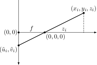Analyzing figure 8.1, it can be observed that the ratios between similar triangles generated by optical rays describe the equation that allows projecting a generic point $(x_{i},y_{i},z_{i})^{\top}$, expressed in camera coordinates (one of the reference systems in which one can operate), into sensor coordinates $(\tilde{u}_{i}, \tilde{v}_{i})^{\top}$:

$$\begin{bmatrix} \tilde{u}_{i} \\ \tilde{v}_{i} \end{bmatrix} = \frac{f}{z_{i}} \begin{bmatrix} x_{i} \\ y_{i} \end{bmatrix}$$ (8.1)

where $f$ is the focal length (the distance between the pin-hole and the sensor). It should be noted that the coordinates $(x_{i},y_{i},z_{i})^{\top}$, expressed in camera coordinates, in this book follow the left-hand rule (commonly used in computer graphics), as opposed to the right-hand rule (more commonly used in robotic applications), which is chosen to express world coordinates. The use of coordinate $z$ to express distance is a purely mathematical requirement due to the transformations that will be presented shortly.

The sensor coordinates $(\tilde{u}_{i}, \tilde{v}_{i})^{\top}$ are not the image coordinates but are still considered "intermediate" coordinates. Therefore, it is necessary to apply an additional transformation to obtain the image coordinates:

$$\begin{bmatrix} u_{i} \\ v_{i} \end{bmatrix} = \begin{bmatr... ... \end{bmatrix} + \begin{bmatrix} u_{0} \\ v_{0} \end{bmatrix}$$ (8.2)

where the coordinates $(u_{0}, v_{0})$ (principal point) account for the offset of the origin of the coordinates in the stored image relative to the projection of the focal point onto the sensor.

$D_{u}$ and $D_{v}$ are conversion factors between the units of the sensor's reference system (meters) and those of the image (pixels), accounting for the various conversion factors involved. With the advent of digital sensors, it is typically $D_{u} = D_{v}$.

In the absence of information available from the various datasheets regarding $f$, $D_{u}$, and $D_{v}$, there is a tendency to consolidate these variables into two new variables referred to as $k_u$ and $k_v$, which represent the effective focal lengths measured in pixels. These can be empirically obtained from the images, as will be discussed in the calibration section. These variables, involved in the conversion between sensor coordinates and image coordinates, are related to each other as

$$\begin{array}{l} k_{u} = D_{u} f = \frac{u_0}{ \tan { \alpha... ..._{v} = D_{v} f = \frac{v_0}{ \tan { \alpha_{v} } } \end{array}$$ (8.3)

with $\alpha_{u}$ and $\alpha_{v}$ angles that can be approximated to the half-angle of the camera aperture (horizontal and vertical, respectively). When the optics are undistorted and the sensor has square pixels, $k_u$ and $k_v$ tend to take on the same value.

Due to the presence of the ratio, the equation (8.1) cannot be clearly represented in a linear system. However, it is possible to modify this representation by adding an unknown $\lambda$ and an additional constraint, allowing us to express this equation in the form of a linear system. To achieve this, we will leverage the theory presented in section 1.4 regarding homogeneous coordinates.

Using homogeneous coordinates, it can be easily shown that the system (8.1) can be written as

$$\begin{bmatrix} \lambda~u_{i} \\ \lambda~v_{i} \\ \lambda ... ...{K} \begin{bmatrix} x_{i} \\ y_{i} \\ z_{i} \\ \end{bmatrix}$$ (8.4)

solved for $\lambda = z_{i}$. For this reason, $\lambda$ is implied, and instead, homogeneous coordinates are used: to obtain the point in non-homogeneous coordinates, one must divide the first two coordinates by the third, resulting in equation (8.1). The use of homogeneous coordinates allows for the implicit representation of division by the coordinate $z$.

The matrix $\mathbf{K}$, combining the transformations (8.2) and (8.3), can be expressed as:

$$\mathbf{K} = \begin{bmatrix} \dfrac{ u_0 }{ \tan { \alpha_{u... ...} & u_{0} \\ 0 & k_{v} & v_{0} \\ 0 & 0 & 1 \\ \end{bmatrix}$$ (8.5)

Such a matrix, not depending, as we will see later, on factors other than those of the chamber itself, is referred to as the matrix of intrinsic factors. The matrix $\mathbf{K}$ is an upper triangular matrix, defined by 5 parameters.

With modern digital sensors and the construction of cameras not manually but with precise numerical control machines, it is possible to set the skew factor $k_{\gamma}$, a factor that accounts for the fact that the angle between the axes in the sensor is not exactly 90 degrees, to zero.

Setting $k_{\gamma}=0$, the inverse of the matrix (8.5) can be expressed as:

$$\mathbf{K}^{-1} = \begin{bmatrix} \dfrac{1}{k_{u}} & 0 & -\d... ...{k_{v}} & -\dfrac{v_{0}}{k_{v}} \\ 0 & 0 & 1 \\ \end{bmatrix}$$ (8.6)

The knowledge of these parameters (see section 8.5 regarding calibration) determines the ability to transform a point from camera coordinates to image coordinates or, conversely, to generate the line in camera coordinates corresponding to a point in the image.

With this modeling, in any case, the contributions due to lens distortion have not been taken into account. The pin-hole camera model is indeed valid only if the image coordinates used refer to undistorted images.

Footnotes

... relationships^8.1

Most models fall under the pinhole model, understood as a model where all light rays pass through a single point; however, there are models that generalize the pinhole model to catadioptric cameras, such as the Mei model, or other different models like the double sphere.