Pin-Hole Camera

This chapter addresses the problem of describing the process through which the light incident on objects is recorded by a digital sensor. This concept is fundamental in image processing, as it provides the relationship linking image points to their position in the world; in other words, it makes it possible to determine the region of the world associated with an image pixel or, conversely, to identify the area of the image that captures a given region in world coordinates.

The universally accepted projective model, known as the Pin-Hole Camera model, is based on simple geometric relationships^9.1.

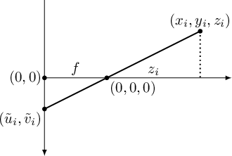
Figure 9.1 shows a highly simplified diagram of how the image is formed on the sensor. The observed point $(x_i,y_i,z_i)^{\top}$, expressed in camera coordinates, is projected onto the sensor plane. All these rays pass through the same point: the projection center (pin-hole).

Figure: The pin-hole camera model. A world point expressed in camera coordinates is projected onto the image plane.

Analyzing Figure 9.1, we observe that the ratios between the similar triangles formed by the optical rays yield the equation that projects a generic point $(x_i,y_i,z_i)^{\top}$, expressed in camera coordinates (one of the reference frames in which operations can be performed), onto the sensor plane:

$$\begin{bmatrix} \tilde{u}_i \\ \tilde{v}_i \end{bmatrix}= \frac{f}{z_i} \begin{bmatrix} x_i \\ y_i \end{bmatrix},$$ (9.1)

where $f$ is the focal length, that is, the distance between the pin-hole and the sensor.

It should be noted that the coordinates $(x_i,y_i,z_i)^{\top}$, expressed in camera coordinates, follow the left-hand rule in this book (widely used in computer graphics), as opposed to the right-hand rule (more commonly used in robotic applications), which is instead used for expressing world coordinates. The coordinate $z_i$ therefore represents the point's depth along the camera's optical axis.

Defining

$$\tilde{x}_i = \frac{x_i}{z_i}, \qquad \tilde{y}_i = \frac{y_i}{z_i},$$ (9.2)

the coordinates $(\tilde{x}_i,\tilde{y}_i)$ are called normalized image coordinates. They represent the intersection of the optical ray with the image plane located at unit distance from the projection center and are independent of the camera's intrinsic parameters, the image resolution, and the physical dimensions of the sensor.

Equation (9.1) can therefore also be written as

$$\begin{bmatrix} \tilde{u}_i \\ \tilde{v}_i \end{bmatrix}= f \begin{bmatrix} \tilde{x}_i \\ \tilde{y}_i \end{bmatrix}.$$ (9.3)

Normalized coordinates thus constitute an intermediate space between the three-dimensional geometry of the scene and the discrete image coordinates. Many computer vision algorithms, such as pose estimation, triangulation, and epipolar geometry, assume that image points are expressed in this reference frame.

The sensor coordinates $(\tilde{u}_i,\tilde{v}_i)^{\top}$ are not yet the coordinates of the digital image, but rather “intermediate” coordinates expressed in the physical units of the sensor. An additional transformation is therefore required to obtain the image coordinates:

$$\begin{bmatrix} u_i \\ v_i \end{bmatrix}= \begin{bmatrix} D... ...v}_i \end{bmatrix}+ \begin{bmatrix} u_0 \\ v_0 \end{bmatrix},$$ (9.4)

where the coordinates $(u_0,v_0)$ (principal point) account for the offset between the origin of the coordinates in the stored image and the projection of the optical center onto the sensor.

$D_u$ and $D_v$ are conversion factors between the units of the sensor reference frame, typically expressed in metric units, and those of the image, expressed in pixels. For square pixels, the two conversion factors are equal.

In the absence of information (available in the various datasheets) about $f$, $D_u$, and $D_v$, these variables are often combined into two new parameters called $k_u$ and $k_v$, namely the effective focal lengths measured in pixels, which can be obtained empirically from images, as discussed in the section on calibration.

These variables are defined as

$$\begin{array}{l} k_u = D_u f, \\ k_v = D_v f. \end{array}$$ (9.5)

Using normalized image coordinates, the transformation to pixel coordinates therefore becomes

$$\begin{array}{l} u_i = k_u \tilde{x}_i + u_0, \\ v_i = k_v \tilde{y}_i + v_0. \end{array}$$ (9.6)

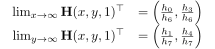
When the principal point approximately coincides with the image center, $k_u$ and $k_v$ can also be related to half the field of view:

$$k_u \simeq \frac{W}{2\tan\alpha_u}, \qquad k_v \simeq \frac{H}{2\tan\alpha_v},$$ (9.7)

where $W$ and $H$ are the image width and height in pixels, respectively, while $\alpha_u$ and $\alpha_v$ are half the horizontal and vertical fields of view, respectively.

When the sensor has square pixels, $k_u$ and $k_v$ tend to have the same value.

Because of the division by $z_i$, Equation (9.1) cannot be represented directly by a linear transformation in Cartesian coordinates. However, it is possible to reformulate it by introducing a scale factor $\lambda$, thereby representing the projection through a linear system in homogeneous coordinates. To do so, we will use the theory presented in Section 1.5 concerning homogeneous coordinates.

The transformation between normalized image coordinates and pixel coordinates can be represented by the intrinsic-parameter matrix

$$\mathbf{K} = \begin{bmatrix} k_u & k_{\gamma} & u_0 \\ 0 & k_v & v_0 \\ 0 & 0 & 1 \end{bmatrix},$$ (9.8)

where $k_{\gamma}$ is the skew factor, which accounts for any non-orthogonality between the sensor axes.

When $k_{\gamma}=0$, we therefore have

$$\begin{bmatrix} u_i \\ v_i \\ 1 \end{bmatrix}= \mathbf{K} \begin{bmatrix} \tilde{x}_i \\ \tilde{y}_i \\ 1 \end{bmatrix}.$$ (9.9)

Recalling that

$$\tilde{x}_i = \frac{x_i}{z_i}, \qquad \tilde{y}_i = \frac{y_i}{z_i},$$

the projection can be written directly in homogeneous coordinates as

$$\begin{bmatrix} \lambda u_i \\ \lambda v_i \\ \lambda \end... ... \mathbf{K} \begin{bmatrix} x_i \\ y_i \\ z_i \end{bmatrix},$$ (9.10)

with $\lambda = z_i$.

For this reason, $\lambda$ is normally omitted and homogeneous coordinates are used: to obtain the point in non-homogeneous coordinates, it is sufficient to divide the first two coordinates by the third. The use of homogeneous coordinates therefore makes the division by coordinate $z_i$ implicit.

Matrix $\mathbf{K}$ depends exclusively on the camera's internal parameters and is therefore called the intrinsic-parameter matrix. In the general case, it is an upper-triangular matrix defined by five parameters.

With modern digital sensors, it is normally possible to set the skew factor $k_{\gamma}$, which accounts for the possibility that the angle between the sensor axes may not be exactly $90^\circ$, to zero.

Setting $k_{\gamma}=0$, the inverse of matrix (9.8) can be written as

$$\mathbf{K}^{-1} = \begin{bmatrix} \dfrac{1}{k_u} & 0 & -\dfr... ...dfrac{1}{k_v} & -\dfrac{v_0}{k_v} \\ 0 & 0 & 1 \end{bmatrix}.$$ (9.11)

In particular, the inverse intrinsic matrix makes it possible to transform an image point into the corresponding normalized image coordinates:

$$\begin{bmatrix} \tilde{x}_i \\ \tilde{y}_i \\ 1 \end{bmatr... ...athbf{K}^{-1} \begin{bmatrix} u_i \\ v_i \\ 1 \end{bmatrix}.$$ (9.12)

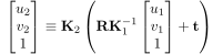
Knowledge of these parameters (see Section 9.5 on calibration) therefore makes it possible to transform a point from camera coordinates to image coordinates or, conversely, to generate the line in camera coordinates associated with an image point. In particular, the vector

$$\begin{bmatrix} \tilde{x}_i \\ \tilde{y}_i \\ 1 \end{bmatrix}$$ (9.13)

identifies, up to a scale factor, the direction of the optical ray associated with image point $(u_i,v_i)$.

This model, however, does not account for the effects of lens distortion. The pin-hole camera model is valid only when the image coordinates used refer to distortion-free images.

Footnotes

... relationships^9.1

Most models fall under the pin-hole model, understood as a model in which all light rays pass through the same point. However, there are models that generalize the pin-hole model to catadioptric cameras, such as the Mei model, as well as other different models, such as the double sphere model.