Lens Distortion

All commercial cameras deviate from the pin-hole camera model, and this deviation is generally greater as the camera's field of view increases: since every optical system consists of a number of lenses, distortion arises from nonidealities during the manufacturing and assembly of the optical system. Producing a distortion-free lens is in fact an extremely costly process, and the problem is particularly evident in low-cost applications, which must rely on inexpensive optics.

These nonidealities produce nonlinear distortion that is difficult to model and, also because this distortion depends on the interaction between the lens and the sensor, lens manufacturers normally do not provide, or are unable to provide, geometric information describing how to represent it.

It is important to note that the pin-hole camera model is valid only when the image being processed is undistorted; therefore, calibration, that is, correction of geometric distortion, is a prerequisite for accurately reconstructing the three-dimensional structure of the observed scene.

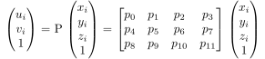
From the optical-ray perspective, the distortion introduced by the lens lies between the world and the pin-hole. The pin-hole camera equation modified to include optical distortion becomes

$$\mathbf{p} = \mathbf{K} f_d( [\mathbf{Rt}]\mathbf{x} )$$ (9.14)

With this formalism, distortion $f_d$ transforms a point from undistorted coordinates to distorted coordinates. This choice, as opposed to the inverse formulation, follows from purely practical considerations: since the objective is to obtain a dense, undistorted output image (see the discussion in Section 1.13), it is necessary to compute the function that transforms an undistorted point into a distorted point.

In general, the lens-distortion contributions are divided into radial components (directed along the line connecting the point to the distortion center) and tangential components (perpendicular to that line). Tangential contributions (as well as other contributions not discussed here) are normally small, whereas radial distortion is always detectable and generally increases in magnitude as the focal length decreases.

This section derives a general relationship between the ideal point $(x,y)$ and the actual observed distorted image point $(\breve{x},\breve{y})$.

There is a single point $(x_d,y_d)$ in the entire image, called the distortion center, at which distortion has no effect. For this point $(x,y)=(\breve{x},\breve{y})$.

To define distortion, it is necessary to work in a new coordinate system centered at the distortion center:

$$\begin{array}{l} \bar{x} = x - x_d \\ \bar{y} = y - y_d \\ \end{array}$$ (9.15)

The distortion center is normally close to $(0,0)$, but there is no guarantee that it coincides with the principal point. Several papers propose, as an approximation, ignoring the distortion center and identifying it with the principal point, or considering only the decentering distortion term.

The classical Brown-Conrady formulation (Bro66) models lens distortion as an offset:

$$\begin{array}{l} \breve{x} = x + \delta_x (\bar{x},\bar{y}) \\ \breve{y} = y + \delta_y (\bar{x},\bar{y}) \end{array}$$ (9.16)

These offsets can be divided into contributions:

radial distortion

The offset due to radial distortion is given by

$$\begin{array}{l} \delta^{r}_x = \bar{x} f_r ( r ) \\ \delta^{r}_y = \bar{y} f_r ( r ) \\ \end{array}$$ (9.17)

where $f_r(r)$ is a function only of the radius 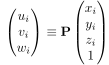$r = \sqrt{\bar{x}^{2}+\bar{y}^{2} }$, the Euclidean distance between the point and the distortion center, subject to the constraint $f_r (0) = 1$.

The function $f_r(r)$ of radial distortion is not known explicitly but can be approximated using the first terms of its series expansion:

$$f_r(r) = 1 + k_{1} r^{2} + k_{2} r^{4} + k_{3} r^{6} + \ldots$$ (9.18)

The presence of only powers that are multiples of 2 is due to the symmetry of function $f_r$.

thin prism distortion

manufacturing imperfections and misalignment between the sensor and the lens introduce additional asymmetric distortions. They are usually modeled as

$$\begin{array}{l} \delta^{(p)}_x = s_1 r^2 + s_3 r^{4} + \ldo... ... \delta^{(p)}_y = s_2 r^2 + s_4 r^{4} + \ldots \\ \end{array}$$ (9.19)

These contributions are often insufficient, however, to describe the effects of optical decentering.

decentering distortion

This is normally caused by incorrect assembly of the lens and the various components that make up the optical system. The Brown-Conrady model represents the decentering contribution as

$$\begin{array}{l} \delta^{(t)}_x = (p_1 (r^2 + 2 \bar{x}^2) +... ...2) + 2 p_1 \bar{x} \bar{y} ) (1 + p_3 r^2 + \ldots) \end{array}$$ (9.20)

This contribution consists of both a radial and a tangential component.

Substituting all these contributions into Equation (9.16), the complete Brown-Conrady model is written as

$$\begin{array}{l} \bar{x} = x - x_d \\ \bar{y} = y - y_d \... ...) (1 + p_3 r^{2} + \ldots) + s_2 r^{2} + \ldots \\ \end{array}$$ (9.21)

In practice, radial distortion is dominant and, in most applications, the first terms are more than sufficient.

For example, OpenCV models distortion using the R3P1 model: three radial terms ($k_1$, $k_2$, $k_3$) and the first-order decentering terms ($p_1$, $p_2$).

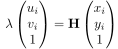
Distortion coefficients are obtained using various techniques available in the literature, applied to images acquired in a structured environment (calibration grids). A nonlinear optimizer is normally used, either by working with lines and iterating until all image curves become straight lines, the plumb-line method (DF01), or by constraining points on a plane with known coordinates to form a homography. These techniques can be applied only when working in image coordinates (approach 1).

To calibrate distortion in normalized camera coordinates (approach 2), the distortion and the camera's intrinsic parameters must be computed simultaneously (Zha99). An initial estimate of the intrinsic parameters can be obtained using a linear optimizer, but the final estimate can be obtained only through a nonlinear optimizer.

The widely used technique for estimating distortion parameters is to optimize the observation of feature points in the image whose positions in world coordinates are known, thereby enforcing a complete perspective projection (Section 9.5.6).