Classification

Classification and machine learning techniques play a predominant role in Computer Vision. Video sensors produce a significantly larger amount of data than most other sensors. This abundance of information is both an opportunity and a challenge, since it requires advanced algorithms capable of extracting meaningful content from it.

As stated earlier, statistics, classification, and model fitting can in fact be viewed as different aspects of a single subject. Statistics seeks the most correct approach from a Bayesian perspective for extracting the hidden parameters (of the state or model) of a system, possibly affected by noise, attempting, given the inputs, to return the most probable output, whereas classification proposes techniques and methods for modeling the system efficiently. Finally, if the exact model underlying a physical system were known, any classification problem could be reduced to an optimization problem. For these reasons, it is therefore not easy, let alone straightforward, to determine where one subject ends and the other begins.

The classification problem consists in deriving the parameters of a generic model that allows the problem to be generalized using a limited number of examples.

A classifier can be viewed in two ways, depending on the type of information that the system is intended to provide:

1. as a “likelihood” function relative to a model, as in equation (5.1);
2. as a partition of the input space, as in equation (5.2).

In the first case, a classifier is represented by a generic function

$$f: \mathbb{R}^{n} \to \mathbb{R}^{m}$$ (5.1)

that associates with the input element $\mathbf {x}$, consisting of the 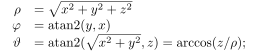$n$ features representing the example to be classified, confidence values for the possible $\{y_1,\ldots,y_m\}$ output classes (categories):

$$f(\mathbf{x}) = \left( p(y_1\vert\mathbf{x}), \ldots, p(y_m\vert\mathbf{x}) \right)$$

that is, the probability that the observed object is precisely $y_i$ given the observed quantity $\mathbf {x}$.

Because of both the infinite number of possible functions and the lack of further specific information about the form of the problem, the function $f$ cannot be a uniquely specified function, but is instead represented by a parametric model of the form

$$\mathbf{y} = f(\mathbf{x}, \boldsymbol\beta)$$

where $\mathbf{y} \in \mathbb{R}^{m}$ is the output space, $\mathbf{x}\in\mathbb{R}^{n}$ is the input space, and $\boldsymbol\beta$ are the parameters of model $f$ to be determined during training.

The training phase is based on a set of examples (training set) consisting of pairs $(\mathbf{x}_i, \mathbf{y}_i)$. Using these examples, the training phase must determine the parameters $\boldsymbol\beta$ of function $f(\mathbf{x},\boldsymbol\beta)$ that minimize, according to a given metric (cost function), the error on the training set itself.

To train the classifier, it is therefore necessary to identify the optimal parameters $\boldsymbol\beta$ that minimize the error in the output space: classification is also an optimization problem. For this reason, machine learning, model fitting, and statistics are closely related research fields. The same considerations used for Kalman or Hough methods, as well as everything discussed in the chapter on least-squares model fitting, can be used for classification, while specific classification algorithms can, for example, be used to fit a set of noisy observations to a curve.

It is normally impossible to produce a complete training set: it is not always possible to obtain every type of input-output association so as to systematically map the entire input space into the output space and, even if this were possible, storing the memory required to represent these associations as a Look Up Table would still be costly. These are the main reasons for using models in classification.

The fact that the training set cannot cover all possible input-output combinations, together with the generation of a model optimized for such incomplete data, can prevent the training from generalizing: elements not present in the training set may be classified incorrectly because of excessive adaptation to the training set (the overfitting problem). This phenomenon is normally caused by an optimization phase that focuses more on reducing the error on the outputs than on generalizing the problem.

Returning to the ways of viewing a classifier, it is often simpler and more generalizable to derive directly from the input data a surface in $\mathbb{R}^n$ that separates the categories in the n-dimensional input space. A new function $g$ can be defined that associates one and only one output label with each group of inputs, in the form

$$g: \mathbb{R}^{n} \to \mathbb{Y}=\{y_1, \ldots, y_m \}$$ (5.2)

This is the second way of viewing a classifier.

Expression (5.1) can always be converted into form (5.2) through majority voting:

$$g(\mathbf{x}) = \argmax_{y_i} p(y_i\vert\mathbf{x})$$ (5.3)

From this perspective, the classifier is a function that directly returns the symbol most similar to the supplied input. The training set must now associate each input (each element of the space) with one and only one output class $y \in \mathbb{Y}$. This way of viewing a classifier usually reduces computational complexity and resource usage.

If function (5.1) actually represents a transfer function, or a response, function (5.2) can be viewed as a partition of space $\mathbb{R}^{n}$ in which each region—generally very complex and not contiguous in the input space—is associated with a single class.

For the reasons given above, it is not physically possible to implement an optimal classifier (except for problems of very limited size or for simple, perfectly known models), but several general-purpose classifiers exist that may be considered suboptimal depending on the problem and the required performance. For classifiers (5.2), the problem is to obtain an optimal partition of the space; consequently, a set of fast primitives that do not use too much memory is required when $n$ has large values, whereas in case (5.1) an explicitly defined function is required that models the problem very accurately while avoiding specialization.

The information (features) that can be extracted from an image to enable its classification is varied. In general, directly using pixel intensity or color values is rare in practical applications, since these values are strongly influenced by the scene's lighting conditions. Moreover, directly representing the image produces a feature space of very high dimensionality, making the learning and classification problem more complex. It is therefore necessary to extract essential information (features) from the image region to be classified, describing its appearance as accurately as possible. For this reason, all the theory presented in section 7 is widely used in machine learning. Both Haar features, thanks to their high extraction speed, and Histograms of Oriented Gradients (HOG, sec. 7.2), thanks to their accuracy, are widely used. As a compromise, and at the same time as a generalization of these two families of features, Integral Channel Features (ICF, sec. 7.3) have been proposed.

To reduce the complexity of the classification problem, it can be divided into several layers to be handled independently: a first layer transforms the input space into the feature space, while a second layer performs the actual classification starting from the feature space.

From this perspective, classification techniques can be divided into three main categories:

Rule-based learning

In this case, both the feature space and the parameters of the classification function are chosen by a human user, without using any data set or training examples;

Machine Learning

The transformation from the input space to the feature space is chosen by the user from a finite set of functions, while the model parameters are extracted by the computer by analyzing the supplied examples;

Representation learning

Both the transformation into the feature space and the extraction of the model parameters are performed by the computer.

Recently, Representation learning techniques built from multiple layers arranged in cascade (Deep Learning) have achieved considerable success in solving complex classification problems.

Among the techniques for transforming the input space into the feature space, PCA, an unsupervised linear technique, is important. Principal Component Analysis (section 2.9.1) is a technique that reduces the number of inputs to the classifier by removing linearly dependent or irrelevant components, thereby reducing the dimensionality of the problem while attempting to preserve as much information as possible.

As for models and general-purpose modeling techniques, the most widely used are

Regression

Regression consists in estimating one or more continuous variables from a set of observations. Many of the modeling techniques presented in chapter 4 can be used for both regression and classification problems by appropriately adapting the cost function and the representation of the outputs.

Neural Network

Neural networks can generate functions of type (5.1) by concatenating sums, multiplications, and strongly nonlinear functions such as sigmoids. Regression techniques can be used to estimate the parameters of this generic model;

Bayesian Classifiers

Bayes' theorem can be used directly as a classifier or to combine several classifiers so as to maximize the a posteriori probability of identifying the correct class (section 5.2);

Decision Tree

in which classifiers are cascaded with other classifiers (and each node represents some attribute extracted from the input data);

Decision Stump

a degenerate decision tree (one node), which partitions the feature space using a simple threshold, thus becoming the simplest (5.2) classifier and an example of a weak classifier;

Ensemble Learning

Multiple weak classifiers (weak) can be combined (Ensemble Learning, section 5.8) so as to maximize some global metric (for example, the separation margin between classes). Strictly speaking, these are not classifiers in their own right, but techniques for combining multiple simple classifiers to generate a complex classifier (ensemble).

Figure: Example of Template Matching. The approach works well on the source image, but cannot be extended to other images, especially in the presence of significant variations in brightness and scale.