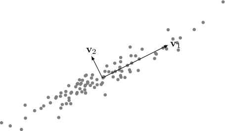
Next: ZCA Up: Eigenvalue Analysis Previous: Eigenvalue Analysis
Principal Component Analysis, or the discrete Karhunen–Loeve transform KLT, is a technique with two important applications in data analysis:
Similarly, there are two formulations of the PCA definition:
A practical example of dimensionality reduction is the equation of a hyperplane in  dimensions: there exists a basis of the space that transforms the equation of the plane, reducing it to
  dimensions without loss of information, thereby reducing the dimensionality of the problem by one.
are stored in the rows2.2 of the matrix  of dimensions
  , a matrix that therefore stores
  random vectors of dimensionality and with
  .
.
Each row corresponds to a different observation  , and the distribution of these experiments must have zero mean, at least empirically.
Assuming that the points have zero mean (which can always be achieved simply by subtracting the centroid), the covariance matrix of the observations is given by
 |
(2.69) |
If the input data  are correlated, the covariance matrix
 is not diagonal.
The goal of PCA is to find an optimal transformation  that transforms correlated data into decorrelated data
 |
(2.70) |
and orders them according to their information content so that, by selecting a subset of the bases, the dimensionality of the problem can be reduced.
If there exists an orthonormal basis such that the covariance matrix
expressed in this basis is diagonal, then the axes of this new basis are called the principal components of
(or of the distribution of ).
When a covariance matrix is obtained whose only nonzero elements are those on the diagonal, the events are mutually uncorrelated in this new basis.
This transformation can be found by solving an eigenvalue problem: it can be shown that the elements of the diagonal matrix are the eigenvalues of
and that the variances of the projections of the vector onto the principal components coincide with these eigenvalues:
where is the eigenvector matrix (an orthogonal matrix such that
 ) and
) and
 is the diagonal matrix of the ordered eigenvalues
 .
.
There are two approaches to obtaining this result.
Since
is a real symmetric positive semidefinite matrix, it can be decomposed as
called the spectral decomposition, where is the orthonormal eigenvector matrix and
is the diagonal eigenvalue matrix. Since the matrix
is positive semidefinite, all eigenvalues are nonnegative.
This technique, however, requires the explicit computation of
.
Given a rectangular matrix , the singular value decomposition (SVD) provides, in a numerically stable manner, the eigenvectors of
 and, through the squares of the singular values, the corresponding eigenvalues.
The SVD is therefore the standard technique for computing principal components.
and, through the squares of the singular values, the corresponding eigenvalues.
The SVD is therefore the standard technique for computing principal components.
Using the SVD, the event matrix can be decomposed as

using the Economy/Compact SVD representation, where  contains the left singular vectors (left singular vectors),
  contains the singular values of , and contains the right singular vectors.
It should be noted that when using the SVD, it is not necessary to compute the covariance matrix
explicitly. This matrix can subsequently be obtained from
 |
(2.73) |
Comparing this relation with equation (2.72) gives
 |
(2.74) |
The following properties of eigenvalues and singular values should be recalled:
 and
share the same nonzero eigenvalues.
and
share the same nonzero eigenvalues.
 of the matrix are the square roots of the eigenvalues of
:
of the matrix are the square roots of the eigenvalues of
:

An important property of the SVD should also be recalled:
which represents the best rank- approximation of the matrix in the Frobenius-norm sense.
This fact, together with the property of the SVD that it returns the singular values in descending order, makes it possible to approximate a matrix with one of lower rank.
approximation of the matrix in the Frobenius-norm sense.
This fact, together with the property of the SVD that it returns the singular values in descending order, makes it possible to approximate a matrix with one of lower rank.
By selecting the eigenvectors associated with the largest eigenvalues, it is possible to construct a matrix

whose columns form an orthonormal basis of the reduced space. The projection of a vector

onto this subspace is

with

The vector  represents a reduced-dimensionality description of the data that preserves most of the variance present in the system.
rather than , and vice versa.