Restricted Boltzmann Machines

Figure 5.9: Restricted Boltzmann Machines.

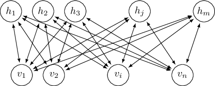
The turning point between shallow and deep training techniques is generally considered to have occurred in 2006, when Hinton and others at the University of Toronto introduced Deep Belief Networks (DBNs) (HOT06), an algorithm that “greedily” trains a layered structure by training one layer at a time using an unsupervised training algorithm. The distinctive feature of DBNs is that their layers consist of Restricted Boltzmann Machines (RBMs) (FH94,Smo86).

Let $\mathbf{v} \in \{0,1\}^{n}$ be a binary stochastic variable associated with the visible state and $\mathbf{h} \in \{0,1\}^{m}$ a binary stochastic variable associated with the hidden state. Given a state $(\mathbf{v}, \mathbf{h})$, the energy of the configuration of the visible and hidden layers is given by (Hop82)

$$E(\mathbf{v}, \mathbf{h} ) = - \sum_{i=1}^{n} a_i v_i - \su... ...1}^{m} b_j h_j - \sum_{i=1}^{n} \sum_{j=1}^{m} w_{i,j} v_i h_j$$ (5.111)

where $v_i$ and $h_j$ are the binary states of the visible and hidden layers, respectively, while $a_i$ and $b_j$ are the weights, and $w_{i,j}$ are the weights associated with them. A Boltzmann Machine is similar to a Hopfield network, except that all outputs are stochastic. The Boltzmann Machine can therefore be defined as a special case of an Ising model, which in turn is a special case of a Markov Random Field. Similarly, RBMs can be interpreted as stochastic neural networks in which the nodes and connections correspond to neurons and synapses, respectively.

The probability of the joint configuration of the visible states $\mathbf{v}$ and hidden states $\mathbf{h}$, parameterized by the vectors $\mathbf{a}$, $\mathbf{b}$ and the weight matrix $\mathbf{W}$, is given by the Boltzmann distribution:

$$P(\mathbf{v}, \mathbf{h} ) = \frac{1}{Z(\cdot)} e^{-E(\mathbf{v}, \mathbf{h}) }$$ (5.112)

where the partition function $Z$ is given by

$$Z=\sum_{\mathbf{v}, \mathbf{h}} e^{-E(\mathbf{v}, \mathbf{h}) }$$ (5.113)

the sum of the energies of all possible pairs of visible and hidden states.

The word restricted refers to the fact that direct interactions between units belonging to the same layer are not allowed; interactions are permitted only between adjacent layers.

Given an input $\mathbf{v}$, the hidden binary state $h_j$ is activated with probability:

$$p(h_j = 1 \vert \mathbf{v}) = \sigma \left( b_j + \sum_i v_i w_{i,j} \right)$$ (5.114)

where $\sigma(x)$ is the logistic function $1 / (1 + exp(-x) )$. Similarly, it is easy to obtain the visible state given the hidden state:

$$p(v_i = 1 \vert \mathbf{h}) = \sigma \left( a_i + \sum_j h_i w_{i,j} \right)$$ (5.115)

Estimating the model parameters $(\mathbf{a}, \mathbf{b}, \mathbf{W})$ so as to correctly model the training-data distribution is computationally expensive. However, in 2002 Hinton proposed the Contrastive Divergence (CD) algorithm, which enables much more efficient training of RBMs, finally making them suitable for large-scale applications. A detailed and practical description of RBM training can be found in (Hin12).