SVM

Figure 5.3: Separating hyperplane between two classes obtained using SVM. The points on the margin (dashed line) are the Support Vectors.

Both LDA and logistic regression yield a linear decision boundary. However, the criteria used to determine this boundary are fundamentally different.

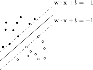
SVM (CV95), like LDA and logistic regression, yields a linear classifier based on a discriminant function of the form shown in equation (5.5). However, the approach is different. The objective of SVM is to determine, among all hyperplanes that correctly separate the two classes, the one that maximizes the separation margin between the training examples and the decision boundary (decision boundary). The underlying idea is that a wider margin generally leads to better classifier generalization and greater robustness to variations in the data.

Let the classification classes be defined as those typical of a binary problem, in the form $y_i \in \{+1,-1\}$, and consider the hyperplane in equation (5.4). Suppose that there exist optimal parameters $(\mathbf{w}_0,b_0)$ satisfying the constraint

$$\begin{array}{ll} \mathbf{x}_i \cdot \mathbf{w}_0 + b_0 \ge... ...athbf{w}_0 + b_0 \leq -1 & \text{per } y_i = -1 \\ \end{array}$$ (5.26)

or, more compactly:

$$y_i ( \mathbf{x}_i \cdot \mathbf{w}_0 + b_0 ) - 1 \geq 0$$ (5.27)

for every $(y_i, \mathbf{x}_i)$ sample provided during training.

It may be assumed that, for each category, one or more vectors $\mathbf{x}_i$ exist for which constraint (5.27) is satisfied with equality. These elements are called Support Vectors. They are the samples that determine the separation margin and, as will be shown later using the KKT conditions, are the only samples associated with nonzero Lagrange multipliers.

The point-to-plane distance $\rho$ (see eq.(1.88)) is

$$\rho = \frac{ \Vert \mathbf{w} \cdot \mathbf{x} + b \Vert } { \Vert \mathbf{w} \Vert }$$ (5.28)

Given two points from opposite classes satisfying equality (5.27), the margin can be derived from equation (5.28) and is

$$\rho = \frac{2}{\Vert \mathbf{w}_0 \Vert}$$ (5.29)

To maximize the margin $\rho$ in equation (5.29), its reciprocal must be minimized, namely,

$$\min_{\mathbf{w},b} \frac{1}{2} \Vert \mathbf{w} \Vert^2$$ (5.30)

subject to the set of constraints expressed by inequality (5.27). This is the standard-form primal optimization problem for SVMs.

This class of problems (minimization subject to inequality constraints, or the primal optimization problem) is solved using the Karush-Kuhn-Tucker approach, which generalizes the method of Lagrange multipliers to inequalities. The KKT conditions yield the Lagrangian function:

$$\mathcal{L}(\mathbf{w}, b, \boldsymbol\alpha) = \frac{1}{2}... ...i \left( y_i ( \mathbf{x}_i \cdot \mathbf{w} + b ) - 1 \right)$$ (5.31)

to be minimized with respect to $\mathbf{w}$ and $b$ and maximized with respect to $\boldsymbol\alpha$. The weights $\alpha_i \geq 0$ are the Lagrange multipliers. Setting the partial derivatives to zero gives

$$\frac{\partial \mathcal{L} }{\partial b} = 0 \rightarrow \sum y_i \alpha_i = 0$$ (5.32)

$$\frac{\partial \mathcal{L}}{\partial \mathbf{w}} = 0 \rightarrow \mathbf{w} = \sum \alpha_i y_i \mathbf{x}_i$$ (5.33)

Substituting these results (the primal variables) into the Lagrangian (5.31) gives a function of the multipliers alone, the dual variables, yielding the Wolfe dual formulation:

$$\Psi (\boldsymbol\alpha) = \sum \alpha_i -\frac{1}{2} \sum_... ...um_j \alpha_i \alpha_j y_i y_j \mathbf{x}_i \cdot \mathbf{x}_j$$ (5.34)

subject to the constraints $\alpha_i \ge 0$ and $\sum \alpha_i y_i = 0$. The maximum of function $\Psi$ computed over $\boldsymbol\alpha$ gives the $\alpha_i$ associated with each training vector $\mathbf{x}_i$. This maximum provides the solution to the original problem.

The KKT conditions apply to this formulation, including the particularly important constraint known as Complementary slackness:

$$\alpha_i \left( y_i ( \mathbf{x}_i \cdot \mathbf{w} + b ) - 1 \right) = 0$$ (5.35)

The complementary slackness condition states that, at the optimum, for each sample, at least one of the multiplier $\alpha_i$ and the constraint violation must be zero. In particular,

$$\alpha_i > 0 \quad\Longrightarrow\quad y_i(\mathbf{x}_i\cdot\mathbf{w}+b)=1$$ (5.36)

Samples associated with nonzero multipliers therefore lie exactly on the margin and are called Support Vectors. All other samples have $\alpha_i=0$ and do not contribute directly to the solution.

By solving the quadratic problem (5.34), subject to constraint (5.32) and $\alpha_i \geq 0$, the weights for which $\alpha_i\neq 0$ holds will be the Support Vectors. Substituting these weights into equations (5.33) and (5.35) yields the maximum-margin hyperplane.

The most widely used method for solving this QP is Sequential Minimal Optimization (SMO). For an in-depth treatment of SVM-related topics, see (SS02).