Decision Trees

Figure 5.4: Example of a Decision Stump. $v$ is a feature extracted from the image and $\theta$ is a threshold.

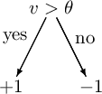
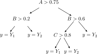
A Decision Tree (Decision Tree) is a very simple and effective method for constructing a classifier, and training decision trees is one of the most successful techniques currently available. A decision tree is a tree of classifiers (Decision Stumps) in which each internal node is associated with a particular “question” about a feature (feature). As many branches as there are possible values of the feature extend from this node, eventually reaching the leaves, which indicate the category associated with the decision. Special attention is generally paid to binary decision nodes.

A good “question” divides samples from heterogeneous classes into subsets with sufficiently homogeneous labels, stratifying the data so that each stratum has low variance.

Figure 5.5: Example of a Decision Tree.

To achieve this, it is necessary to define a metric that measures this impurity. Let $X$ be a subset of samples from a particular training set consisting of $m$ possible classes. $X$ is in fact a random variable that takes only discrete values (the continuous case is analogous). Each discrete value $x_i$, which can take $X$, can be associated with the probability distribution $p(x_i) = p_i$. $X$ is a data set consisting of $m$ classes, and $p_i$ is the relative frequency of class $i$ within the set $X$.

Figure 5.6: Comparison of impurity measures for a binary classification problem.

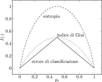
Given the definition of $X$, the following metrics are widely used in decision trees:

Entropy

From information theory, the entropy $I_H$ of $X$ is:

$$I_H(X)=-\sum_{i=1}^{m} p_i \log_2 p_i$$ (5.73)

Gini Index

The Gini impurity index is defined as

$$I_G(X) = 1 - \sum_{i=1}^m{p^2_i}$$ (5.74)

Classification Error

From Bayesian theory:

$$I_E(X) = 1 - \max_i{p_i}$$ (5.75)

Intuitively, a node with class distribution $(0,1)$ has minimum impurity, whereas a node with a uniform distribution $(0.5,0.5)$ has maximum impurity.

A “question” $h_j(x)$, with $k$ possible answers, divides the set $\mathcal{E}$ into the subsets $\mathcal{E}_1, \ldots, \mathcal{E}_k$.

To assess how well the condition performs, the impurity of the child nodes must be compared with that of the parent node: the greater the difference, the better the selected condition.

Given a metric $I(\cdot)$ that measures impurity, the gain $\Delta$ is a criterion that can be used to determine the quality of the split:

$$\Delta = I(\mathcal{E}) - \sum_{i=1}^{k} \frac{ N(\mathcal{E}_i) } { N(\mathcal{E}) } I( \mathcal{E}_i)$$ (5.76)

where $N(\mathcal{E})$ is the number of samples in the parent node and $N(\mathcal{E}_i)$ is the number of samples in the i-th child node.

When entropy is used as the metric, the gain $\Delta$ is known as Information Gain (TSK06).

Decision trees induce algorithms that choose a test condition maximizing the gain $\Delta$. Since $I(\mathcal{E})$ is the same for all possible classifiers and $N(\mathcal{E})$ is constant, maximizing the gain is equivalent to minimizing the weighted sum of the impurities of the child nodes:

$$\hat{h} = \argmin_{h_j} \sum_{i=1}^{k} N(\mathcal{E}_i) I( \mathcal{E}_i)$$ (5.77)

The best question $h_j(x)$ is the one that minimizes this quantity.

For binary classifiers, the Gini metric is widely used, since the gain to be minimized reduces to

$$\frac{p_1 n_1}{p_1 + n_1} + \frac{p_2 n_2}{p_2 + n_2}$$ (5.78)

where $p_1,n_1$ is the number of positive and negative samples that the classifier moves to the left branch and $p_2,n_2$ is the number of samples in the right branch.

Decision trees adapt very well and quickly to the training data and consequently, if unrestricted, systematically suffer from overfitting. A refinement algorithm (pruning) is normally applied to trees to reduce the problem of overfitting wherever possible. There are usually two pruning approaches: pre-pruning and post-pruning. Pre-pruning stops tree growth under certain conditions to avoid excessive specialization, for example, by imposing a maximum tree depth. Post-pruning, on the other hand, refines an already constructed tree by removing branches that fail to satisfy certain conditions on a previously selected validation set.

This technique for constructing a decision tree is usually referred to as Classification and regression trees (CART) (B$^+$84). In the realistic case where the analyzed features are statistical quantities, one does not speak of creating a classification tree, but rather of constructing a regression tree. Finding the optimal partition of the data is an NP-complete problem; therefore, greedy algorithms such as the one shown in the section are normally used.