AdaBoost and its variants

Figure 5.7: Comparison of loss functions: 0/1-loss, logistic, exponential, and quadratic

The Boosting problem can be generalized and viewed as a problem in which one must find predictors $f_t(\mathbf{x})$ that minimize the global cost function:

$$\sum_{i=1}^{m} \phi \left( y_i \left( f_1(\mathbf{x}_i) + \ldots + f_n(\mathbf{x}_i) \right) \right)$$ (5.92)

where $\phi \in \mathcal{C}^1$ is a convex, non-increasing function of $\lim_{z \to \infty} \phi(z)=0$.

From an analytical perspective, AdaBoost is an example of a coordinate-wise gradient descent optimizer that minimizes the potential function $\phi(z)=e^{-z}$, optimizing one coefficient $\alpha_t$ at a time (LS10), as shown in equation (5.81).

The following is a non-exhaustive list of AdaBoost variants that highlights some of the distinctive features of this technique:

AdaBoost with abstention

AdaBoost can also be extended to classifiers with abstention, for which the possible outputs are $h_j(x_i) \in \{-1,0,+1\}$. By extending definition (5.84), let $W_{-}$ denote failures, $W_{0}$ abstentions, and $W_{+}$ successes of classifier $h_t$.

In this case as well, $Z_t$ reaches its minimum at the same value of $\alpha_t$ as in the case without abstention; see (5.90), and with this choice $Z_t$ would be

$$Z_t = W_0 + 2 \sqrt{ W_{-} W_{+}}$$ (5.93)

However, a more conservative choice of $\alpha_t$ was proposed by Freund and Schapire:

$$\alpha_t = \frac{1}{2} \log \left( \frac{W_{+} + 1/2 W_0}{W_{-} + 1/2 W_0} \right)$$ (5.94)

which makes it possible to establish an upper bound on $Z_t$.

Real AdaBoost

Real AdaBoost generalizes the preceding case and, above all, generalizes the same extended additive model (FHT00). Rather than using dichotomous hypotheses $h_t(x)$ and assigning them a weight $\alpha_t$, it directly seeks the feature $f_t(x)$ that minimizes equation (5.81).

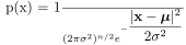Real AdaBoost makes it possible to use weak classifiers that provide the probability distribution $p_t(x) = P[y=1 \vert x, w^{(t)} ] \in [0,1]$, namely the probability that class $y$ is actually $+1$ given observation of feature $x$.

Given a probability distribution $p_t(x)$, the feature $f_t(x)$ that minimizes equation (5.81) is

$$f_t(x) = \frac{1}{2} \log \frac{ P [y=+1 \vert x, w^{(t)} ] ... ...vert x, w^{(t)} ] } = \frac{1}{2} \log \frac{p_t(x)}{1-p_t(x)}$$ (5.95)

This result is equal to half of the logistic transformation. Since the objective remains to minimize the exponential cost function, the weight update remains the one in equation (5.87). Both Discrete and Real AdaBoost, by choosing a weak classifier that satisfies equation 5.95, cause AdaBoost to converge asymptotically to

$$\lim_{T \to \infty} F_T(x) = \frac{1}{2} \log \frac{P[y=+1\vert x]}{P[y=-1\vert x]}$$ (5.96)

showing that the AdaBoost algorithm is an iterative procedure that combines several weak classifiers to approximate a Bayesian classifier.

Real AdaBoost can also be used with a discrete classifier such as the Decision Stump. By applying equation (5.95) directly to the two possible output states of the Decision Stump (it is nevertheless easy to obtain the minimum of $Z_t$ algebraically), the classifier responses must take the values

$$f(x) = \left\{ \begin{array}{ll} \frac{1}{2} \log \frac{W_... ...\log \frac{W_{FN}}{W_{TN}} & x \leq \theta \end{array}\right.$$ (5.97)

with values $W_{*}$, namely the sums of the weights associated with False Positives (FP), False Negatives (FN), True Positives (TP), and True Negatives (TN). With this choice of values, $Z_t$ assumes the notable value

$$Z_t = 2 \left( \sqrt{W_{TP}W_{FP}} + \sqrt{W_{FN}W_{TN}} \right)$$ (5.98)

which is the metric to use when selecting the best feature $x$ and threshold $\theta$.

Gentle AdaBoost

The weights associated with outliers in Real AdaBoost can become very large because of the logarithm in the equation. In this case, it is useful to make the regression more “gentle.”

Gentle AdaBoost further generalizes the concept of Ensemble Learning to an additive model (FHT00) by using regression with the steps typical of Newton methods:

$$F_{T+1}(x) = F_T(x) + f_t(x) = F_T(x) + \E_{w^{(t)}} [ y \vert x ]$$ (5.99)

The hypothesis $f_t(x)$, to be added to the additive model at iteration $t$, is selected from all possible hypotheses $f_k$ as the one that optimizes a weighted least-squares regression:

$$f_t = \argmin_{f_k} \sum_i w_i (y_i - f_k(x_i))^2$$ (5.100)

but at each iteration the AdaBoost weight update is used (5.87), namely the exponential cost function. Gentle AdaBoost can also be used with the Decision Stump. In this case, the minimum of (5.100) in the decision algorithm takes the notable form

$$f(x) = \left\{ \begin{array}{ll} \frac{W_{TP} - W_{FP} }{ ... ..._{TN} }{ W_{TN} + W_{FN} } & x \leq \theta \end{array}\right.$$ (5.101)

LogitBoost

For historical reasons, AdaBoost did not originate from an explicit probabilistic formulation. A first observation is that the classifier output does not directly represent a probability: the value produced by the combination of weak classifiers can in fact take any real value and is not limited to the interval $[0,1]$.

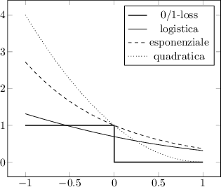
Moreover, the cost function minimized by AdaBoost does not derive directly from a maximum-likelihood principle, as is the case in many statistical models. However, it can be shown that the exponential function used by AdaBoost provides a good approximation to logistic loss and that the classifier can be interpreted as an additive model for estimating probabilities.

This observation naturally leads to logistic regression and to the definition of boosting algorithms derived from statistical criteria. In particular, LogitBoost constructs an additive model by directly optimizing the likelihood of a Bernoulli model.

Additive logistic regression takes the form

$$\log \frac{P(y=+1\vert x)} {P(y=-1\vert x)} = F_T(x) = \sum_{t=1}^{T} f_t(x)$$ (5.102)

where $F_T(x)$ represents the sum of the weak classifiers generated during the boosting process.

Inverting the preceding relation gives

$$p(x) = P(y=+1\vert x) = \frac{e^{F_T(x)}} {1+e^{F_T(x)}} = \frac{1} {1+e^{-F_T(x)}}$$ (5.103)

which associates a probability with the additive model $F_T(x)$.

The objective of training is therefore to estimate the function $F_T(x)$ by maximizing the likelihood of the Bernoulli model. This problem is equivalent to minimizing the log-loss:

$$L = \sum_{i=1}^{N} \log\!\left( 1+\exp\!\left(-y_iF_T(x_i)\right) \right).$$ (5.104)

LogitBoost iteratively constructs the additive model using Newton steps applied to the log-likelihood. At each iteration, a working response and a set of weights obtained from the current probability estimate are introduced:

$$z_i = \frac{y_i^{*}-p(x_i)} {p(x_i)\left(1-p(x_i)\right)}$$ (5.105)

$$w_i = p(x_i)\left(1-p(x_i)\right)$$ (5.106)

where

$$y_i^{*}\in\{0,1\}.$$ (5.107)

The weak hypothesis $f_t(x)$ is then obtained by weighted least-squares regression of the variable 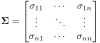$z_i$ with respect to the observations $x_i$, using the weights $w_i$. After each iteration, the additive function is updated and a new probability estimate is calculated using equation (5.103).

Unlike AdaBoost, which originated as an adaptive resampling method and only subsequently received a statistical interpretation, LogitBoost derives directly from a probabilistic model and explicitly optimizes the Bernoulli log-likelihood.

Asymmetric-AdaBoost

Asymmetric-AdaBoost introduces a variant of the weight-update rule (VJ01). The problem with AdaBoost is that it does not allow direct control over the weight assigned to classification errors in the different classes, nor does it allow the number of false positives to be minimized explicitly, but only the classification error. The Asymmetric-AdaBoost variants instead modify, at each iteration $t$, the weights associated with positive and negative samples by cost factors $c^{(t)}_{+}$ and $c^{(t)}_{-}$, respectively.

Cascade

The weight assigned to a classifier is set to $\alpha_t = - \log \beta_t$, twice the weight assigned by AdaBoost.M1.

MAdaBoost

The MAdaBoost algorithm uses a different weight update to reduce the contribution of outliers (or overly complex examples) during training. The maximum weight $w^{(t)}_i$ that a sample can assume is upper-bounded by $w^{(0)}_i$, the value assigned to the weight at the beginning of the algorithm.

This behavior can be represented by a cost function of the form

$$\phi(z)=\left\{\begin{array}{ll} 1-z & z \leq 0 \\ e^{-z} & z > 0 \\ \end{array}\right.$$ (5.108)