Sampson Error

Figure 4.1: Between a manifold $\mathcal {V}$ and a point $\mathbf {p}$, one can identify the point at minimum geometric distance $\hat {\mathbf {p}}$ and the point determined by the Sampson distance $\mathbf {x}$.

In many data-regression problems, it is necessary to have a metric for determining how far an $\mathbf {p}$ is from the actual model. For this purpose, it would be useful to have an $\hat {\mathbf {p}}$ estimate of the observation without the noise component, that is, a datum that belongs exactly to the model. Neither of these quantities can normally be obtained directly without introducing unknown auxiliary variables. It is nevertheless possible to estimate these values by linearizing the model function in the neighborhood of the observation.

Let $\mathbf {p}$ be a noisy observation and let $f(\mathbf{x})=\mathbf{0}$ be a multidimensional manifold representing a particular model to which the observation must belong, namely $\mathbf{p} = \hat{\mathbf{p}} + \epsilon$.

The residual $f(\mathbf{p})$ is an algebraic measure of the proximity between the point and the model and provides no useful information in absolute terms: if the function is replaced by a nonzero multiple of itself, it obviously represents the same locus of points, but the value of the function changes accordingly. From the perspective of the maximum-likelihood estimator, under additive white Gaussian noise on the observations, the correct metric is the geometric distance between the point $\mathbf {p}$ and the point $\hat {\mathbf {p}}$ belonging to the model, that is, estimating $\epsilon$.

We therefore examine the problem of computing an approximate distance between the point $\mathbf{p} \in \mathbb{R}^m$ and a geometric manifold $f(\mathbf{x})=\mathbf{0}$, where $f: \mathbb{R}^{m} \mapsto \mathbb{R}^{n}$ is a differentiable function in a neighborhood of $\mathbf {p}$.

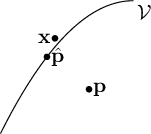
The point $\hat {\mathbf {p}}$ on the manifold that is closest to the point $\mathbf {p}$ is, by definition, the point that minimizes the geometric error

$$\hat{\mathbf{p}} = \argmin_\mathbf{x} \Vert \mathbf{p} - \mathbf{x} \Vert$$ (4.60)

subject to the constraint $f(\mathbf{x})=0$ (or $\min \vert\vert \epsilon \vert\vert^2$ subject to the constraint $f(\mathbf{p} + \epsilon)=\mathbf{0}$).

The difference between minimizing a quantity algebraically and linearly and minimizing a geometric quantity nonlinearly prompted the search for a possible compromise. The Sampson method, initially developed for manifolds such as conics, requires an assumption that can instead be applied to several problems: the derivatives of the cost function in the neighborhood of the minimum $\hat {\mathbf {p}}$ must be approximately linear and therefore approximable through a series expansion. The manifold $f(\mathbf{p})=0$ can be approximated using Taylor expansion so that

$$\tilde{f}(\mathbf{x}) \approx f(\mathbf{p}) + \mathbf{J}_f \boldsymbol\delta_{\mathbf{x}} = \mathbf{0}$$ (4.61)

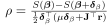with $\mathbf{J}_f$ the $n \times m$ matrix of the Jacobian of the function $f$ evaluated at $\mathbf {p}$ and $\boldsymbol\delta_{\mathbf{x}} = \mathbf{x}-\mathbf{p}$.

This is the equation of a hyperplane in $\mathbf {x}$, and the distance between the point $\mathbf {p}$ and the plane 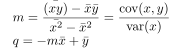$\tilde{f}(\mathbf{x})=0$ is the Sampson distance, or the approximate maximum likelihood (AML). The Sampson error represents the geometric distance between the point and the first-order approximation of the function (geometric distance to first order approximation function).

The problem now becomes that of finding the point $\mathbf {x}$ closest to $\mathbf {p}$, that is, minimizing $\Vert\boldsymbol\delta_{\mathbf{x}}\Vert$ subject to the linear constraint

$$\mathbf{J}_f \boldsymbol\delta_{\mathbf{x}} = -f(\mathbf{p})$$ (4.62)

As this is a constrained minimization problem, it is solved using Lagrange multipliers, yielding the notable result

$$\boldsymbol\delta_{\mathbf{x}} = - \mathbf{J}^{\top} \left( \mathbf{J} \mathbf{J}^{\top} \right)^{-1} f(\mathbf{p})$$ (4.63)

an interesting result when compared, for example, with the Gauss-Newton method, equation (4.53).

The value $\boldsymbol\delta_\mathbf{x}$ represents an estimate of the distance from the point $\mathbf {p}$ to the manifold and can be used both to determine whether the point belongs to the manifold (for example, within algorithms such as RANSAC to identify outliers) and potentially as an alternative cost function to the Euclidean norm. $\boldsymbol\delta_\mathbf{x}$ is the Sampson error, and its norm, given by

$$\Vert \boldsymbol\delta_x \Vert^2 = \boldsymbol\delta_x^{\t... ...\left( \mathbf{J} \mathbf{J}^{\top} \right)^{-1} f(\mathbf{p})$$ (4.64)

indicates the squared distance between the point and a point on the manifold (or, more precisely, its first-order approximation).

In the notable case $n=1$, the Sampson distance reduces to

$$\Vert \boldsymbol\delta_x \Vert^2 = \dfrac{\left( f(\mathbf{p}) \right)^{2}}{\left\Vert \nabla f(\mathbf{p}) \right\Vert^2}$$ (4.65)

Practical applications of the Sampson error include the distance between a point and a conic (see Section 4.6.7), the distance between a pair of points and a homography, and the distance between a pair of corresponding points with respect to the Fundamental matrix (Section 10.4.2).

The Sampson distance can be generalized to the case of multiple constraints using the Mahalanobis distance, that is, by minimizing

$$\min_\epsilon \sum \vert\vert \epsilon \vert\vert^2_\Sigma ... ...epsilon \sum \epsilon^{\top} \boldsymbol \Sigma^{-1} \epsilon$$ (4.66)

subject to the constraint $f(\mathbf{p}+\epsilon)=0$. The equation above therefore generalizes to

$$\Vert \boldsymbol\delta_x \Vert^2 = \boldsymbol\delta_x^{\t... ...boldsymbol \Sigma \mathbf{J}^{\top} \right)^{-1} f(\mathbf{p})$$ (4.67)