


Next: Newton-Raphson Method Up: Regression and Optimization Methods Previous: Total Least Squares
We now consider a generic unconstrained function-modeling (optimization) problem, applicable, for example, to classification problems in computer vision. The considerations presented in this section apply to least-squares problems but can be extended to a generic loss function.
Let  be the set of data involved in the modeling operation, consisting of pairs
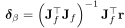 composed of an arbitrary input
  and output
  .
Let
.
Let
 be the cost function (loss function) that returns the quality of the estimate for
 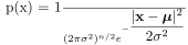 .
The goal is to find the weights
.
The goal is to find the weights
 that parameterize the function
 and minimize a cost function

 .
For simplicity, we will always refer to the latter case, the discrete one, when describing the cost function.
.
For simplicity, we will always refer to the latter case, the discrete one, when describing the cost function.
In the case of additive Gaussian noise, the maximum-likelihood estimator is the quadratic loss function in Equation (4.7):
 |
(4.31) |
In practical applications, it is almost never possible to obtain the minimum of the function in closed form. It is therefore necessary to use suitable iterative methods that start from an initial state and gradually approach the minimum of the objective function by moving along suitable directions
 .
.
