


Next: Optimization on a Manifold Up: Optimization Methods Previous: Sampson Error
When the observation noise is not isotropic, the Euclidean distance can no longer be used to measure the error; instead, it is necessary to use the Mahalanobis distance. Under this different metric, the cost function (4.49) is written as
where
 is the information matrix (information matrix), also called the concentration matrix or precision matrix.
The Mahalanobis distance corresponds to the maximum-likelihood estimator in the case of zero-mean anisotropic Gaussian noise.
In the special case where the covariance matrix is diagonal, this approach reduces to the weighted least-squares case.
is the information matrix (information matrix), also called the concentration matrix or precision matrix.
The Mahalanobis distance corresponds to the maximum-likelihood estimator in the case of zero-mean anisotropic Gaussian noise.
In the special case where the covariance matrix is diagonal, this approach reduces to the weighted least-squares case.
The Taylor-series expansion of equation (4.68) is written as
with 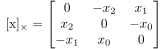 and
and  evaluated at point
 .
The matrix
.
The matrix
 |
(4.70) |
is the information matrix of the entire system, obtained by projecting the measurement error into parameter space through the Jacobian .
For compactness, we also define
 |
(4.71) |
The derivatives of the function  therefore become
Setting the gradient to zero yields the linear system
which represents the Gauss-Newton formulation in the case of anisotropic noise and constitutes the natural generalization of equation (4.52) obtained in the isotropic case.
Paolo medici



