Maximum Likelihood Estimation

When SVD decomposition is used to enforce the constraints, the resulting Fundamental (or Essential) Matrix fully satisfies the requirements for being Fundamental (or Essential), but is merely the matrix closest, under a particular norm—in this case, the Frobenius norm—to the one obtained from the linear system. This solution is therefore not optimal either, since it does not account for how errors propagate from the input points through the transformation: it is still an algebraic rather than a geometric solution.

A first technique that minimizes geometric error consists in exploiting the distance between points and the epipolar lines generated by the Fundamental Matrix (epipolar distance). Even intuitively, the distance between a point $\mathbf {p}_2$ and the epipolar line $\mathbf{F}\mathbf{p}_1$ can be used as a metric for estimating geometric error:

$$d \left( \mathbf{p}_{2}, \mathbf{F} \mathbf{p}_{1} \right) ... ...right)_1^{2} + \left( \mathbf{F}\mathbf{p}_1 \right)_2^{2} } }$$ (10.68)

where $(.)_i$ denotes the $i$-th component of the vector (see section 1.6.3 for the point-to-line distance equation). The smaller the distance, the better matrix $\mathbf{F}$ satisfies the epipolar constraint for the observed correspondences.

Since this error can be computed for both the first and the second image, both contributions should be minimized together. This metric can be used to define a cost function that minimizes the error symmetrically (symmetric transfer error) between the two images:

$$\min_\mathbf{F} \sum_i \left( d\!\left( \mathbf{p}_{1,i}, \... ...\mathbf{p}_{2,i}, \mathbf{F}\mathbf{p}_{1,i} \right)^2 \right)$$ (10.69)

In this case as well, a solution with 8 unknowns can be sought, but obtaining a robust solution requires constraining $\mathbf{F}$ to have rank 2.

As an alternative to the Symmetric Transfer Error, the first-order approximation of the distance between the points and the function (Sampson-error, section 4.3.8) is often used in the literature. An approximate distance between the corresponding image points $\left( \mathbf{p}_{1}, \mathbf{p}_{2} \right)$ and the manifold $\hat{\mathbf{p}_{2}}^{\top}\mathbf{F} \hat{\mathbf{p}_{1} }=0$ can thus be defined using the metric

$$r\left( \mathbf{p}_{1}, \mathbf{p}_{2}, \mathbf{F} \right) ... ... \mathbf{p}_2)_1^2 + (\mathbf{F}^{\top} \mathbf{p}_2)_2^2 } }$$ (10.70)

where $(.)_i$ again denotes the $i$-th component of the vector. Using this approximate metric, while retaining the additional constraint $\det \mathbf{F} = 0$, it is possible to minimize

$$\min_{\mathbf{F}} \sum_{i=1}^{n} r\left( \mathbf{p}_{1,i}, \mathbf{p}_{2,i}, \mathbf{F} \right)^{2}$$ (10.71)

Both the Symmetric Transfer Error and the Sampson distance are better metrics than the algebraic estimate, but neither is the optimal estimator. The Maximum Likelihood Estimation of the Fundamental Matrix would in fact be obtained using a cost function of the form

$$\min_\mathbf{F} \sum_i \Vert \mathbf{p}_{1,i} - \hat{\mathb... ...rt^2 + \Vert \mathbf{p}_{2,i} - \hat{\mathbf{p}}_{2,i} \Vert^2$$ (10.72)

where $\hat{\mathbf{p}}_{1,i}$ and $\hat{\mathbf{p}}_{2,i}$ denote the exact points, and $\mathbf{p}_{1,i}$ and $\mathbf{p}_{2,i}$ the corresponding measured points affected by zero-mean white Gaussian noise. The cost function (10.72) must be minimized subject to the constraint

$$\hat{\mathbf{p}}^{\top}_{2,i} \mathbf{ F } \hat{\mathbf{p}}_{1,i} = 0$$ (10.73)

and to the additional constraints arising from the nature of $\mathbf{F}$. In this case, the exact points $\hat{\mathbf{p}}_{1,i}$ and $\hat{\mathbf{p}}_{2,i}$ become part of the problem (auxiliary variables, subsidiary variables). However, introducing points $\hat{\mathbf{p}}_{1,i}$ and $\hat{\mathbf{p}}_{2,i}$ as unknowns transforms the problem into a nonlinear constrained optimization which, although formally solvable, is inconvenient to address directly.

To solve this problem, the estimation of the Essential or Fundamental Matrix must be combined with three-dimensional reconstruction, using the three-dimensional coordinates of the observed point $\hat{\mathbf{x}}_{i}$ directly as the auxiliary variable. The Essential Matrix can be obtained when the intrinsic parameters of the two sensors are known. In this case, the nonlinear system that projects the auxiliary variable $\hat{\mathbf{x}}_{i}$ onto the respective observations in the two sensors can be used:

$$\begin{array}{l} \hat{\mathbf{p}}_{1,i} \equiv \mathbf{K}_... ...f{R} \hat{\mathbf{x}}_{i} + \mathbf{t} \right) \\ \end{array}$$ (10.74)

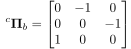
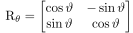
where matrix $\mathbf{R}$ can be expressed through a 3-parameter parameterization (see section A), whereas vector $\mathbf{t}$ must be represented using a 2-parameter parameterization, since the scale remains an unknown factor. By inserting constraints (10.74) into equation (10.72), the objective of recovering the Essential Matrix is transformed into that of directly recovering the relative parameters between the two sensors. If necessary, the Essential Matrix can finally be obtained by directly applying definition (10.43) once the relative pose between the sensors has been determined.

When the intrinsic parameters are unavailable, as in Fundamental Matrix estimation, a true three-dimensional reconstruction of the scene cannot be performed precisely because these parameters are missing. It is nevertheless possible to use fictitious perspective projections by setting $\mathbf{K}_1=\mathbf{I}$ and obtaining constraints of the form:

$$\begin{array}{l} \hat{\mathbf{p}}_{1,i} \equiv \hat{\mathb... ...}_{2,i} \equiv \mathbf{P} \hat{\mathbf{x}}_{i} \\ \end{array}$$ (10.75)

using directly the auxiliary variable $\hat{\mathbf{x}}_{i}$, whose coordinates are therefore known up to an affine transformation 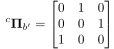$\mathbf{K}_1^{-1}$, namely, the intrinsic parameters of camera 1.

By inserting constraints (10.75) into equation (10.72), the objective of recovering the Fundamental Matrix is again transformed into that of recovering the parameters of the projective matrix 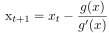$\mathbf{P}$. Using camera matrix $\mathbf{P}=\left[ \mathbf{R}' \vert \mathbf{t}' \right]$, a fictitious camera matrix, it is finally possible to recover $\mathbf{F}$ by directly applying definition (10.43), although matrix $\mathbf{R}'$ is not a rotation matrix.

The probabilistically correct Maximum Likelihood estimate of the Fundamental Matrix nevertheless requires substantial computational resources: in addition to the 11 global unknowns needed to estimate $\mathbf{P}$^10.4 (compared with the 5 for the Essential Matrix), 3 additional unknowns are introduced into the problem for each pair of points to be minimized.

As a final warning, techniques such as RANSAC (section 4.12) are widely used for optimal matrix estimation in the presence of possible outliers in the scene.

Footnotes

...#tex2html_wrap_inline17804#^10.4

From a practical standpoint, 12 coefficients and 11 degrees of freedom