Regression to a Conic

The regression of a parabola, circle, or ellipse can clearly be generalized to any arbitrarily oriented conic (Section 1.7).

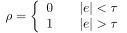Let $(x_i, y_i)^{\top}$, with $i=1, \ldots, n$, be noisy points belonging to the locus to be estimated.

Equation (1.92) can be rewritten in the form

$$\mathbf{a}_i^{\top}\boldsymbol\beta=0$$ (4.115)

where $\mathbf{a}_i=\left\{ x_i^2, x_i y_i, y_i^2, x_i, y_i, 1 \right\}$ and $\boldsymbol\beta=\left\{ a,b,c,d,e,f \right\}$ from which it is clear that the parameters $\boldsymbol\beta$ of any conic can be obtained by solving a homogeneous $\mathbf{A}\boldsymbol\beta=0$ problem in six unknowns, minimizing a quantity of the form

$$S = \sum_{i=1}^{n} \mathbf{a}_i^{\top}\boldsymbol\beta$$ (4.116)

This solution clearly minimizes an algebraic rather than a geometric error and is therefore not the optimal estimator.

An alternative formulation for obtaining the parameters of conics can be found in (FPF99).

Finally, to determine whether a point is close to a conic equation, or to obtain a geometric approximation of the point-to-conic distance, one can compute the Sampson error (Section 4.3.8), exploiting the fact that, for a conic with equation (1.92), the gradient of the manifold has a particularly simple form:

$$\nabla f (x,y) = \left( 2 a x + b y + d, b x + 2 c y + e \right)$$ (4.117)