Gauss-Newton

The methods discussed so far allow considerable freedom in choosing the loss function. In practical cases where the cost function $\ell$ is quadratic, further optimizations can be introduced over Newton's method, avoiding the costly computation of the Hessian.

In this case, the loss function takes the form seen earlier:

$$S(\boldsymbol\beta) = \frac{1}{2} \mathbf{r}^{\top} \mathbf{r} = \frac{1}{2} \sum_{i=1}^{n} r_i^2 (\boldsymbol\beta)$$ (4.49)

The term $1/2$ serves to obtain a more compact expression for the gradient.

With this cost function, the gradient and Hessian are written as:

$$\begin{array}{l} \nabla S(\boldsymbol\beta) = \sum_{i=1}^{... ...athbf{J}_{r} + \sum_{i=1}^{n} r_i \mathbf{H}_{r_i} \end{array}$$ (4.50)

When the parameters are close to the solution, the residual is small and the Hessian can be approximated by its first term:

$$\mathbf{H}_S(\boldsymbol\beta) \approx \mathbf{J}_{r}^{\top}\mathbf{J}_{r}$$ (4.51)

Under these conditions, the gradient and Hessian of the cost function $S$ depend only on the Jacobian of the functions $r_i(\boldsymbol\beta)$. The Hessian approximated in this way can be substituted into equation (4.38):

$$- \mathbf{J}_{r}^{\top} \mathbf{r} = \mathbf{H}_{S} \boldsy... ...ox \mathbf{J}_{r}^{\top}\mathbf{J}_{r} \boldsymbol\delta_\beta$$ (4.52)

As in Newton's method, a linear least-squares problem is obtained, solvable through the normal equations:

$$\boldsymbol\delta_\beta = - \left( \mathbf{J}_{r}^{\top}\mathbf{J}_{r} \right)^{-1} \mathbf{J}_{r}^{\top} \mathbf{r}$$ (4.53)

The geometric meaning of the normal equations is that the minimum is attained when $\mathbf{J}\boldsymbol\delta_\beta - \mathbf{r}$ is orthogonal to the column space of $\mathbf{J}$. In the special case where the residual is written as:

$$r_i = y_i - f_i(\mathbf{x}_i ; \boldsymbol\beta)$$ (4.54)

or as in equation (4.7), it is possible to use $\mathbf{J}_f$, the Jacobian of $f$, instead of $\mathbf{J}_r$:

$$\boldsymbol\delta_\beta = \left( \mathbf{J}_{f}^{\top}\mathbf{J}_{f} \right)^{-1} \mathbf{J}_{f}^{\top} \mathbf{r}$$ (4.55)

having observed that the derivatives of $r_i$ and $f_i(\mathbf{x}_i)$ coincide up to a sign.^4.3

Footnotes

... sign.^4.3

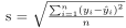The derivatives coincide when a residual of the form $r_i = \hat{y}_i - y_i$ is chosen.