Homographic Transformations

Homogeneous coordinates (Section 1.5) make it possible to represent a very broad range of transformations by unifying linear and affine transformations, such as rotations, translations, and changes of scale, as well as projective transformations, within a single formalism.

A homographic transformation is a one-to-one correspondence between two projective planes that preserves incidence relations between points and lines.

Given two distinct planes $\Pi_i$ and $\Pi_j$, they are said to be related by a homographic transformation (homographic transformation) when there is a one-to-one correspondence between the points of the two planes that preserves incidence relations between points and lines. In particular, each point of $\Pi_i$ corresponds to exactly one point of $\Pi_j$, and each line of $\Pi_i$ corresponds to exactly one line of $\Pi_j$.

Let plane $\Pi$ be observed from two different views. In space $\mathbb{R}^{2}$, the homography (the homographic transformation) is represented by equations of the form:

$$\begin{array}{l} u_j = \dfrac{h_0 u_i + h_1 v_i + h_2}{h_6 ... ...c{h_3 u_i + h_4 v_i + h_5}{h_6 u_i + h_7 v_i + h_8} \end{array}$$ (1.111)

where $(u_i,v_i)$ are the coordinates of points belonging to the projection of plane $\Pi$ in image $i$, whereas $(u_j,v_j)$ are the coordinates of the projections of the same points in image $j$.

Because of its particular form, this transformation can be described through a linear transformation using homogeneous coordinates (Section 1.5):

$$\begin{bmatrix} u_j \\ v_j \\ 1 \end{bmatrix}\sim \mathbf{H}^{\Pi}_{ij} \begin{bmatrix} u_i \\ v_i \\ 1 \end{bmatrix}$$ (1.112)

where

$$\mathbf{H}^{\Pi}_{ij} = \begin{bmatrix} h_0 & h_1 & h_2 \\ h_3 & h_4 & h_5 \\ h_6 & h_7 & h_8 \\ \end{bmatrix}.$$ (1.113)

has been defined. In space $\mathbb{R}^{2}$, homographies are encoded by matrices $3 \times 3$ (2D homographies); similarly, homographic transformations can be defined for higher-dimensional spaces. For compactness, and to retain the reference to a row-major in-memory representation, as in C, matrix $\mathbf{H}^{\Pi}_{ij}$ has been expressed using the coefficients $h_0 \ldots h_8$ rather than the classical syntax for denoting the elements of the matrix.

The homography matrix $\mathbf{H}^{\Pi}_{ij}$ is defined as the matrix that converts homogeneous points $\mathbf{x}_i$ belonging to the projection of plane $\Pi$ in image $i$ into homogeneous points $\mathbf{x}_j$ in image $j$ according to the relation

$$\mathbf{x}_j \sim \mathbf{H}^{\Pi}_{ij} \mathbf{x}_i.$$ (1.114)

Since this is a relation between homogeneous quantities, the system is defined up to a multiplicative factor: any nonzero multiple of the parameters of the homography matrix defines the same transformation, because homogeneous coordinates are themselves defined up to a scale factor. Consequently, the number of degrees of freedom of the problem is not 9 but 8, since an additional constraint can always be imposed on the matrix elements. Commonly used constraints include $h_8 = 1$ and $\Vert \mathbf{H} \Vert _{F}=1$. It should be noted that $h_8 = 1$ is not generally an optimal constraint from a computational standpoint, since the order of magnitude of $h_8$ may be very different from that of the other matrix elements and, when $h_8=0$, this normalization is not possible.

The alternative constraint $\Vert \mathbf{H} \Vert _{F}=1$ does not privilege any particular matrix element and is especially natural when the parameters are obtained through factorizations such as the SVD. Indeed, denoting by $\mathbf{h} = (h_0,\ldots,h_8)^{\top}$ the vector of homography parameters, each point-to-point correspondence provides constraints on the coefficients of $\mathbf{h}$. As will be shown in detail in Section 9.5.1, these constraints can be collected into a homogeneous linear system of the form $\mathbf{A}\mathbf{h}=0$. Since the zero solution is not meaningful, a normalization constraint must be imposed, for example $\Vert\mathbf{h}\Vert=1$, leading exactly to the homogeneous linear-system problem discussed in Section 1.1. In the presence of noise, the solution is obtained by selecting the right singular vector associated with the smallest singular value of matrix $\mathbf{A}$.

Figure 1.6: Example of a homographic transformation: the homography relates planes in perspective to planes that are not in perspective.

Figure 1.7: Example of a homographic transformation: the homography relates “virtual” planes to one another.

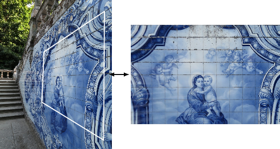
Applications involving homographic transformations are numerous. They will be discussed in detail in Chapter 9 on the pin-hole camera, but, in summary, these transformations make it possible to remove perspective from image planes, project planes in perspective, and associate points on planes observed from different viewpoints. One way to obtain projective transformations is to establish correspondences between points on the planes to be transformed and thereby determine the parameters of the homography matrix (1.111), including in an overdetermined manner, for example through the least-squares method. A method for obtaining the coefficients is shown in equation (9.58). It should be remembered that this transformation, which relates points on planes between two perspective views, applies only to points on the plane under consideration: the homography relates points on a plane to one another, but only those points. Any point not belonging to the plane will be reprojected to an incorrect position.

Since a homographic transformation is represented by a nonsingular matrix, it is invertible, and its inverse is also a homographic transformation:

$$\left( \mathbf{H}^{\Pi}_{ij} \right)^{-1} = \mathbf{H}^{\Pi}_{ji}.$$ (1.115)

One possible form for the inverse of homography (1.111) is

$$\begin{array}{l} u_i = \dfrac{(h_5 h_7 - h_4 h_8)u_j + (h_1... ...u_j + (h_1 h_6 - h_0 h_7) v_j + h_3 h_1 - h_0 h_4 } \end{array}$$ (1.116)

and, since it is known up to a multiplicative factor, it is not necessary to normalize the inverse matrix by its determinant (unnormalized inverse homographic matrix).

It should be noted that when the homography does not introduce a projective component, that is, when $h_6=0 \wedge h_7=0$, the homographic transformation reduces to an affine transformation (affine transformation) represented by the usual equations

$$\begin{array}{l} u_j = h_0 u_i + h_1 v_i + h_2 \\ v_j = h_3 u_i + h_4 v_i + h_5 \end{array}$$ (1.117)

encountered earlier.