The Integral Image

Figure 1.10: Construction of the integral image and use for area calculation.

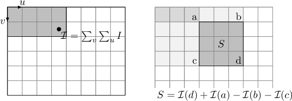
Let $I$ be a generic grayscale image. The value of pixel $(x,y)$ of the integral image $\mathcal{I}$ represents the sum of the values of every pixel of the source image contained within the rectangle $(0,0)-(x,y)$:

$$\mathcal{I}(x,y) = \sum_{v=0}^{y} \sum_{u=0}^{x} I(u,v)$$ (1.99)

With this definition, it is worth noting that the corners of the rectangle are included in the summation (figure 1.10).

The computational trick of using the integral image allows optimization of various algorithms presented in this book, particularly SURF (section 5.4) and the extraction of Haar features (section 6.1).

Thanks to the integral image, it is possible, at a constant computational cost of 4 sums, to obtain the summation of any rectangular sub-region of the image $I$:

$$\begin{array}{l} \sum_{y=y_0}^{y_1} \sum_{x=x_0}^{x_1} I(x... ...- \mathcal{I}(x_1,y_0-1) - \mathcal{I}(x_0-1,y_1) \end{array}$$ (1.100)

The value obtained in this way represents the sum of the elements of the original image within the rectangle (extremes included).

In addition to being able to quickly calculate the summation of any subset of the image, it is also possible to easily obtain convolutions with kernels of a particular shape in a very straightforward manner, while maintaining performance that is invariant with respect to the size of the filter. Examples of convolution masks can be seen in section 6.1.