


Next: MLE computation of the Up: Calibration Previous: Calibration
The basic idea of the Direct Linear Transformation proposed by Abdel-Aziz and Karara (AAK71) makes it possible to directly compute the coefficients of matrices (9.56), (9.59), or of matrix (9.25), completely disregarding the parameters and structure of the perspective-transformation model. That paper also presents an approach for solving overdetermined problems using the pseudoinverse technique.
Given system (9.25), it is necessary to recover the 12 parameters of the projective matrix  to obtain an implicit calibration of the system, that is, one in which the internal parameters (from 9 to 11, depending on the model) that generated the elements of the matrix are unknown. This representation of the pin-hole camera is clearly ideal (with no nonlinearities in the model).
The perspective function written in implicit form is
 are written in row-major order.
It is possible to rearrange system (9.52) to obtain 2 pairs of linear constraints for each point whose image and world coordinates are known:
are written in row-major order.
It is possible to rearrange system (9.52) to obtain 2 pairs of linear constraints for each point whose image and world coordinates are known:
Since this is a homogeneous system, its solution is the null space of
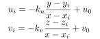 , the kernel of the matrix of known terms. For this reason, matrix is defined only up to a multiplicative factor, and consequently has only 11 free parameters (there are even fewer when considering that a modern camera has only 3–4 intrinsic parameters and 6 extrinsic parameters).
Since the system has been rearranged, noise propagation on the points is no longer linear, and this solution does not satisfy the maximum-likelihood criterion.
The matrix obtained through this procedure, although it conceals the sensor's internal structure, makes it possible to project a point from world coordinates to image coordinates and, from a point in image coordinates, to recover the line subtended by that point in the world.
, the kernel of the matrix of known terms. For this reason, matrix is defined only up to a multiplicative factor, and consequently has only 11 free parameters (there are even fewer when considering that a modern camera has only 3–4 intrinsic parameters and 6 extrinsic parameters).
Since the system has been rearranged, noise propagation on the points is no longer linear, and this solution does not satisfy the maximum-likelihood criterion.
The matrix obtained through this procedure, although it conceals the sensor's internal structure, makes it possible to project a point from world coordinates to image coordinates and, from a point in image coordinates, to recover the line subtended by that point in the world.
The result is generally unstable when only 6 points are used. Therefore, the estimate is normally obtained by processing more than the minimum number of points and using techniques such as the pseudoinverse to determine a solution that minimizes measurement errors.
 :
:
The problem is the same as the one considered previously: the homogeneous solution exists, and the homogeneous solution equation (9.53) generalizes to
 .
.
This formulation is useful when the projective model does not follow the pin-hole model, but it is still possible to recover the “camera” coordinates of the optical rays subtended by the pixel, and therefore available in homogeneous form.
The number of elements in matrix can usually be reduced by imposing the constraint that all points involved in the calibration process belong to a particular plane (for example, the ground plane).
This means imposing the condition 
 , which implies removing one column (the one corresponding to axis
  ) from the matrix,
which is reduced to size
) from the matrix,
which is reduced to size  , becomes invertible, and can be defined as a homography (see Section 1.11).
We therefore define matrix
 (cf. (9.36)) as
As in the previous case, it is possible to transform the nonlinear relation (9.56) to obtain linear constraints:
If a sufficiently modern linear-system solver is available, the additional constraint
 is automatically satisfied while computing the kernel of the matrix of known terms (QR factorization or SVD decomposition).
Another, simpler and more intuitive method consists in imposing the additional constraint 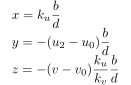 . In this way, instead of solving a homogeneous system, a conventional linear problem can be solved.
System (9.56) can also be rearranged in this case to obtain linear constraints in the form:
. In this way, instead of solving a homogeneous system, a conventional linear problem can be solved.
System (9.56) can also be rearranged in this case to obtain linear constraints in the form:
 , and each point whose position on a plane in the world and position in the image are both known provides 2 constraints.
However, imposing means that point  cannot be an image singularity (e.g., the horizon line), and in general it is not an optimal choice in terms of solution accuracy, as discussed previously.
It is important to note that the solution depends strongly on the chosen normalization. The choice 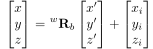 can be called standard least-squares.
In both cases, at least 4 points are required to obtain a homography  , and each additional point makes it possible to obtain a solution with lower error.
When overdetermined, these systems can be solved using the pseudoinverse method 1.1.
, and each additional point makes it possible to obtain a solution with lower error.
When overdetermined, these systems can be solved using the pseudoinverse method 1.1.
Matrix is defined by 4 intrinsic parameters and 6 extrinsic parameters.
Separating the intrinsic parameters from the extrinsic parameters suggests extracting them independently in order to make the calibration more robust.
After all, the intrinsic parameters can be determined offline with a certain degree of accuracy and remain valid for all possible camera positions (see 9.5.4 below).
We define matrix
 (cf. (9.37)) as
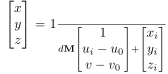 denotes the so-called normalized image coordinates (homogeneous coordinates of point
 in camera coordinates).
Matrix is defined up to a scale factor, whereas
makes it possible to define the scale because it still contains two orthonormal columns.
Knowing the two columns of the rotation matrix makes it possible to recover the third; therefore, this calibration is also valid for points outside plane  .
.
As before, a nonlinear system of 3 homogeneous equations, when suitably rearranged, provides two linear constraints:
 equations for all
  control points in order to determine the 9 unknowns.
The matrix is defined up to a multiplicative factor, but in this case the internal structure of matrix
can help recover the extrinsic parameters (cf. Section 9.5.3).
In fact, the two columns of the matrix must be orthonormal:
control points in order to determine the 9 unknowns.
The matrix is defined up to a multiplicative factor, but in this case the internal structure of matrix
can help recover the extrinsic parameters (cf. Section 9.5.3).
In fact, the two columns of the matrix must be orthonormal:
 |
(9.61) |
Equations (9.53) and (9.57) can also be derived from purely geometric considerations, since the image and camera vectors must be parallel (factor  is purely multiplicative and can affect the vector only through an affine transformation):
 |
(9.62) |
Paolo medici


![\begin{displaymath}
\left[
\begin{array}{ccccccccc}
x_i & y_i & 1 & 0 & 0 & 0 &...
...ight] \begin{pmatrix}
h_0 \\
\vdots \\
h_8
\end{pmatrix} = 0
\end{displaymath}](img1699.svg)


