Essential Matrix and Fundamental Matrix

In 1981, Christopher Longuet-Higgins (Lon81) was the first to observe that a generic point expressed in world coordinates, its corresponding points in camera coordinates, and the pin-holes must be coplanar. The geometric derivation of the relationships between these points is omitted, and the analytical derivation is presented directly.

It has been noted several times that a point in an image subtends a line in space, and that this line, projected onto another image acquired by a camera at a different viewpoint, represents the epipolar line on which the corresponding point from the first image lies. This equation, which relates points in one image to lines in the other, can be expressed in matrix form.

Following Higgins's reasoning, the intrinsic-parameter matrix will be left implicit, and normalized camera coordinates will be used.

Without loss of generality, consider a system consisting of two cameras, with the first positioned and oriented with respect to the second by the projection matrix $\mathbf{P}_1=[\mathbf{R}\vert\mathbf{t}]$, while the second is located at the origin of the reference frame and aligned with the axes, with projection matrix $\mathbf{P}_2=[\mathbf{I}\vert\mathbf{0}]$. The same result can be obtained starting from two generic calibrated cameras, arbitrarily oriented and positioned with respect to a third reference frame, through relationships $\mathbf{R} = \prescript{2}{}{\mathbf{R}}_{1} = \mathbf{R}^{-1}_{2} \mathbf{R}_{1}$ and $\mathbf{t}$, namely, the position of camera 1 with respect to reference frame 2.

A generic point $\mathbf{x} \in \mathbb{R}^3$ has coordinates $\mathbf{x}_1$ and $\mathbf{x}_2$ in the two different reference frames and is projected onto sensors 1 and 2 at the points, expressed in camera coordinates, $\mathbf{m}_1$ and $\mathbf{m}_2$, respectively.

The image point $\mathbf{m}_2$ identifies an optical ray in three-dimensional space passing through the projection center of the second camera. Since this center has been placed at the origin of the reference frame, the ray can be parameterized as

$$\mathbf{x}_2 = \lambda_2 \mathbf{m}_2, \qquad \lambda_2 > 0.$$ (10.38)

A generic point $\mathbf{x}_1 = \lambda_1 \mathbf{m}_1$ expressed in the coordinates of sensor 1 and observed by that sensor can be projected into the coordinates of sensor 2 according to

$$\mathbf{x}_2 = \prescript{2}{}{ \mathbf{R}_1 } \mathbf{x}_1 + \mathbf{t}$$ (10.39)

The equation of the epipolar line, a line in camera coordinates in the second sensor and the locus of points on which $\mathbf{m}_2$ must lie, associated with point $\mathbf{m}_1$ (observed and therefore expressed in the camera coordinates of the first sensor), is

$$\lambda_2 \mathbf{m}_2 = \lambda_1 \prescript{2}{}{ \mathbf{R}_1 } \mathbf{m}_1 + \mathbf{t}$$ (10.40)

The locus of homogeneous points $\mathbf{m}_2$ is obtained by varying parameter $\lambda_1$, and this line in $\mathbb{R}^3$ is also a line in $\mathbb{R}^2$. If two points are indeed corresponding points, the system is solvable and the parameters $\lambda_1$ and $\lambda_2$ can be determined (this is an example of three-dimensional reconstruction by triangulation, as discussed in Section 10.3.1).

There is, however, a relationship between points in the two cameras that eliminates parameters $\lambda$ and, more importantly, makes it possible to reason in the reverse direction, namely, to determine the relative pose between the two cameras $\left( \mathbf{R}, \mathbf{t} \right)$ from a list of corresponding points.

If both sides of equation (10.40) are first multiplied vectorially by $\mathbf{t}$ and then scalarly by $\mathbf{m}^{\top}_{2}$, we obtain

$$\lambda_2 \mathbf{m}^{\top}_{2} \left( \mathbf{t} \times \ma... ...thbf{m}^{\top}_{2} \left( \mathbf{t} \times \mathbf{t} \right)$$ (10.41)

The properties of the cross product $\mathbf{t} \times \mathbf{t}=\textbf{0}$ and dot product $\mathbf{m}_2 \cdot \left( \mathbf{t} \times \mathbf{m}_2 \right)=0$ can be applied to this relationship.

This step has a precise geometric meaning. The resulting relationship expresses the fact that vector $\mathbf{t}$, the optical ray associated with $\mathbf{m}_2$, and the optical ray associated with $\prescript{2}{}{\mathbf{R}_1}\mathbf{m}_1$ lie in the same epipolar plane. In other words, the two projection centers and the observed three-dimensional point are coplanar. The rigidity assumption also makes it possible to relate the coordinates of the same point in the two reference frames through transformation $(\mathbf{R}, \mathbf{t})$.

Using this formula, the relationships between corresponding points $\mathbf{m}_1$ and $\mathbf{m}_2$, represented as homogeneous camera coordinates, can be expressed in the very compact form

$$\mathbf{m}^{\top}_{2} \left( \mathbf{t} \times \mathbf{ R } \mathbf{m}_1 \right) = 0$$ (10.42)

Finally, denoting the skew-symmetric matrix $[\mathbf{t}]_{\times}$, which represents the cross product in matrix form (Section 1.8), the different terms can be collected into the matrix

$$\mathbf{E} = [\mathbf{t}]_{\times} \mathbf{R} = \mathbf{R} \left[ \mathbf{R}^{\top} \mathbf{t} \right]_{\times}$$ (10.43)

where $\mathbf{R}=\prescript{2}{}{\mathbf{R}_1}$ and $\mathbf{t}$ have the meaning introduced in equation (10.39): $\mathbf{R}$ transforms coordinates expressed in the camera 1 reference frame into the camera 2 reference frame, whereas $\mathbf{t}$ represents the position of the optical center of camera 1 expressed in the camera 2 reference frame. This defines a linear relationship linking the camera points in the two views:

$$\mathbf{m}^{\top}_{2} \mathbf{ E } \mathbf{m}_1 = 0$$ (10.44)

Matrix $\mathbf{E}$ is called the Essential Matrix and encodes the relative pose between the two cameras, up to a scale factor on the translation.

Finally, attention must be paid to the conventions adopted, since the literature contains no unique choice for the ordering of points in epipolar relationships. In the case of relationship

$$\mathbf{m}_2^{\top}\mathbf{E}\mathbf{m}_1 = 0,$$

, matrix $\mathbf{E}=[\mathbf{t}]_{\times}\mathbf{R}$ is constructed using rotation $\mathbf{R}$ and translation $\mathbf{t}$, which transform coordinates expressed in the camera 1 reference frame into the camera 2 reference frame.

Matrix $\mathbf{E}$, relating homogeneous points, is also homogeneous and is therefore defined up to a multiplicative factor.

The Essential Matrix has the following properties:

• the transpose of the Essential Matrix for the ordered camera pair (1,2) is (proportional to) the Essential Matrix for the pair (2,1);
• $\mathbf{E}$ is a rank-2 matrix with 5 degrees of freedom. It represents a relative pose and therefore has 3 degrees of freedom associated with rotation and 2 degrees of freedom associated with the direction of the relative translation;
• the two singular values of matrix $\mathbf{E}$ must be equal, and the third must be zero.

defined as the image of the other camera centre)

The Essential Matrix establishes relationships in camera coordinates and therefore, to use it in practice, points expressed in this particular reference frame must be available; that is, the intrinsic parameters of the cameras involved must be known.

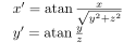
The equation

$$\mathbf{m}^{\top}_{2} \left( \mathbf{ E } \mathbf{m}_1 \right) = 0$$ (10.45)

expresses the epipolar constraint between observations $\mathbf{m}_1$ and $\mathbf{m}_2$ of the same three-dimensional point.

It is nevertheless possible to introduce an additional relationship between image points that does not require explicit knowledge of the cameras' intrinsic parameters.

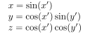
Applying the definition of homogeneous camera coordinates $\mathbf{p} = \mathbf{K} \mathbf{m}$ in relationship (10.44) gives

$$\mathbf{p}^{\top}_2 \mathbf{K}^{-\top}_{2} \mathbf{E} \mathb... ...{1} \mathbf{p}_1 = \mathbf{p}^{\top}_2 \mathbf{F} \mathbf{p}_1$$ (10.46)

from which

$$\mathbf{F} = \mathbf{K}^{-\top}_{2} \mathbf{E} \mathbf{K}^{-1}_{1}$$ (10.47)

The Fundamental Matrix (Fundamental matrix) is defined (Faugeras and Hartley, 1992) as:

$$\mathbf{p}^{\top}_{2} \mathbf{ F } \mathbf{p}_1 = 0$$ (10.48)

where $\mathbf {p}_1$ and $\mathbf {p}_2$ are the homogeneous coordinates of the corresponding points in the first and second images, respectively.

If two points in the two images of the stereo pair represent the same world point, equation (10.48) must be satisfied.

The Fundamental Matrix narrows the search interval for correspondences between the two images because, by point-line duality, relationship (10.48) can be used to specify the locus of points in the second image where the point from the first image must be sought. In fact, the equation of a line on which points $\mathbf {p}_2$ and $\mathbf {p}_1$ must lie is given by

$$\begin{array}{l} \mathbf{l}_2 = \mathbf{F} \mathbf{p}_1 \\ \mathbf{l}_1 = \mathbf{F}^{\top} \mathbf{p}_2 \\ \end{array}$$ (10.49)

where $\mathbf{l}_1$ and $\mathbf{l}_2$ are the parameters of the epipolar line belonging to the first and second images, respectively, written in implicit form.

The relationship between the Fundamental Matrix and the Essential Matrix is, according to equation (10.46),

$$\mathbf{E} = \mathbf{K}^{\top}_{2} \mathbf{F} \mathbf{K}_{1}$$ (10.50)

or, conversely,

$$\mathbf{F} = \mathbf{K}^{-\top}_{2} \mathbf{E} \mathbf{K}^{... ...\top}_{2} [\mathbf{t}]_{\times} \mathbf{R} \mathbf{K}^{-1}_{1}$$ (10.51)

The Essential Matrix depends exclusively on the relative pose between the cameras, whereas the Fundamental Matrix depends on both the intrinsic parameters and the relative pose.

The Essential Matrix introduces constraints identical to those of the Fundamental Matrix but, although it was historically introduced before the Fundamental Matrix, it is a special case of the latter because it expresses the relationships in camera coordinates.

$\mathbf{F}$ is a $3 \times 3$ rank-2 matrix, and 7 points are sufficient to determine it, since it has only 7 degrees of freedom (a multiplicative factor and the zero determinant reduce the dimensionality of the problem). The relationship between the Fundamental Matrix and its 7 degrees of freedom is nonlinear^10.1. With (at least) 8 points, however, a linear estimate of the matrix can be obtained, as described in the next section.

The Fundamental Matrix has the following properties:

• the transpose of the Fundamental Matrix for the ordered camera pair (1,2) is the Fundamental Matrix for the pair (2,1);
• $\mathbf{F}$ is a rank-2 matrix with 7 degrees of freedom (the homogeneous matrix $\mathbf{F}$ has 8 degrees of freedom, to which the constraint $\det \mathbf{F} = 0$ must be added);
• $\mathbf{l}_2 = \mathbf{F} \mathbf{p}_1$ and $\mathbf{l}_1 = \mathbf{F}^{\top} \mathbf{p}_2$ are the epipolar lines in image 2 of a point in image 1 and in image 1 of a point in image 2, respectively;
• since the epipoles satisfy relationships $\mathbf{F}\mathbf{e}_1=0$ and $\mathbf{F}^{\top}\mathbf{e}_2=0$, epipole $\mathbf {e}_1$ belongs to the right null space of matrix $\mathbf{F}$, whereas epipole $\mathbf {e}_2$ belongs to the left null space;
• $\mathbf{F}$ is a “quasi-correlation”, that is, a transformation that maps points to lines but is not invertible.

Figure 10.3: The Fundamental Matrix identifies the epipolar lines, right image, on which the corresponding points of points in the left image lie.

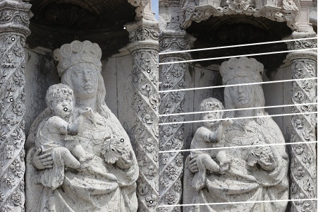
The Fundamental and Essential Matrices can be used to narrow the search for corresponding points between two images and/or filter out possible outliers (for example, in RANSAC). Decomposing the Essential Matrix makes it possible to recover the relative pose between the two cameras^10.2, thereby providing an approximate indication of the motion undergone by a camera moving through the world (motion stereo) or of the relative pose of two cameras in a stereo pair (relative auto-calibration).

Using the Essential Matrix makes it possible to recover the relative pose between two views. However, the length of the baseline joining the two pin-holes cannot be determined; only its direction can be recovered. Nevertheless, given the Essential Matrix, it is always possible to reconstruct the observed scene three-dimensionally up to a multiplicative factor: the ratios between distances are known, but not their absolute values. When the same scene is observed from more than two different views, this makes it possible to obtain a consistent three-dimensional reconstruction in which the unknown multiplicative factor remains the same for all views, thereby allowing all the individual reconstructions to be fused into a single reconstruction known up to the same scale factor.

Footnotes

... nonlinear^10.1

The constraint $\det(\mathbf F)=0$ introduces a nonlinear cubic relationship between the elements of the matrix.

... cameras^10.2

As will be seen later, in fact, four configurations are obtained, and the translation is known only up to a multiplicative factor