


Next: Reconstruction with Rectified Cameras Up: Three-Dimensional Reconstruction Previous: Three-Dimensional Reconstruction
|
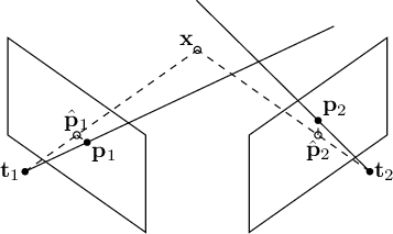
From Figure 10.2, it is easy to see that the solution to the triangulation problem is the intersection point of the epipolar lines generated by the two images.
This problem can readily be extended to the case of 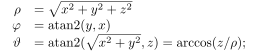 cameras whose relative pose is known. If the relative pose is unknown, it can be obtained, up to a scale factor, directly from the images using techniques such as the Essential matrix (Section 10.4).
Because of inaccuracies in identifying corresponding points (calibration errors could also be considered separately), the lines formed by the optical rays are generally skew.
In this case, it is necessary to derive the closest solution under some cost function: the least-squares solution is always possible with 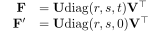 , using techniques such as Forward Intersections or the Direct Linear Transform (DLT).
Every optical ray subtended by image pixel  , with
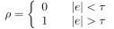 denoting view i, must satisfy equation (10.9).
The intersection point (Forward Intersections) of all these rays is the solution of a potentially overdetermined linear system with
denoting view i, must satisfy equation (10.9).
The intersection point (Forward Intersections) of all these rays is the solution of a potentially overdetermined linear system with  unknowns in
  equations:
 |
(10.13) |
 denotes the direction vector of the optical ray in world coordinates.
The unknowns are the world point to be estimated,
denotes the direction vector of the optical ray in world coordinates.
The unknowns are the world point to be estimated,  , and the depth parameters
  along the respective optical rays.
The closed-form solution, limited to the case of only two lines, is given in Section 1.6.8. This technique can be applied to the case of one camera aligned with the axes and a second camera positioned relative to the first according to relationship (10.5).
Using the properties of the cross product, the same expression can be obtained using perspective projection matrices and image points expressed as homogeneous coordinates:
![\begin{displaymath}
\left\{
\begin{array}{l}
\left[ \mathbf{p}_{1} \right]_{\tim...
...right]_{\times} \mathbf{P}_n \mathbf{x} = 0
\end{array}\right.
\end{displaymath}](img1793.svg) |
(10.14) |
![$[\cdot]_{\times}$](img1794.svg) is the cross product written in matrix form.
Each of these constraints provides three equations, but only two are linearly independent. All these constraints can finally be rearranged into a homogeneous system of the form
is the cross product written in matrix form.
Each of these constraints provides three equations, but only two are linearly independent. All these constraints can finally be rearranged into a homogeneous system of the form
 is a matrix
  with denoting the number of views in which point is observed.
The solution of homogeneous system (10.15) can be obtained through singular value decomposition.
This approach is called the Direct Linear Transform (DLT), by analogy with the calibration technique.
with denoting the number of views in which point is observed.
The solution of homogeneous system (10.15) can be obtained through singular value decomposition.
This approach is called the Direct Linear Transform (DLT), by analogy with the calibration technique.
Minimization in world coordinates, however, is not optimal in terms of noise minimization.
In the absence of additional information about the structure of the observed scene, the optimal estimate (Maximum Likelihood Estimation) is always the one that minimizes the error in image coordinates (reprojection), but it requires greater computational cost and the use of nonlinear techniques, since the cost function to be minimized is
 |
(10.16) |
 and
and  is the projection matrix of the i-th image (Figure 10.2).
This is a non-linear, non-convex problem: potentially several local minima are present, and the linear solution must be used as the starting point for the minimization.
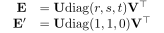
An alternative approach consists of estimating the relative pose between two cameras using the Essential matrix. Once this pose is known, the observed three-dimensional points can be reconstructed by triangulation, as shown in Section 10.4.4.


