Homographic Transformations

The homogeneous coordinates (section 1.4) allow for the representation of a very broad spectrum of transformations, unifying under the same formalism both linear transformations (affine, rotations, translations) and perspective transformations.

Given two distinct planes $\Pi_i$ and $\Pi_j$, they are said to be related by a homographic transformation (homographic transformation) when there exists a one-to-one correspondence such that:

• to each point or each line of $\Pi_i$ corresponds exactly one point and one line of $\Pi_i$
• to each bundle of lines of $\Pi_j$ corresponds a projective bundle on $\Pi_j$

Let the plane $\Pi$ be observed from two different views. In the space $\mathbb{R}^{2}$, the homography (the projective transformation) is represented by equations of the type:

$$\begin{array}{l} u_j = \dfrac{h_0 u_i + h_1 v_i + h_2}{h_6 ... ...c{h_3 u_i + h_4 v_i + h_5}{h_6 u_i + h_7 v_i + h_8} \end{array}$$ (1.75)

where $(u_i,v_i)$ are coordinates of points belonging to the plane $\Pi_i$, while $(u_j,v_j)$ are points of the plane $\Pi_j$.

Due to its particular form, this transformation can be described through a linear transformation using homogeneous coordinates (section 1.4):

$$\begin{bmatrix} u_j \\ v_j \\ 1 \end{bmatrix}= \mathbf{H}^{\Pi}_{ij} \begin{bmatrix} u_i \\ v_i \\ 1 \end{bmatrix}$$ (1.76)

having defined

$$\mathbf{H}^{\Pi}_{ij} = \begin{bmatrix} h_0 & h_1 & h_2 \\ h_3 & h_4 & h_5 \\ h_6 & h_7 & h_8 \\ \end{bmatrix}$$ (1.77)

In space $\mathbb{R}^{2}$, homographies are encoded by matrices $3 \times 3$ (2D homographies): in the same way, projective transformations can be defined for higher-dimensional spaces. For compactness and to maintain reference to a memory representation in row-major, as in C, the matrix $\mathbf{H}^{\Pi}_{ij}$ has been expressed using coefficients $h_0 \ldots h_8$ rather than the classical syntax to indicate the elements of the matrix.

The homographic matrix $\mathbf{H}^{\Pi}_{ij}$ is defined as the matrix that converts homogeneous points $\mathbf{x}_i$ belonging to the plane $\Pi_i$ of the image $i$ into homogeneous points $\mathbf{x}_j$ of the image $j$ with the relationship

$$\mathbf{x}_j = \mathbf{H}^{\Pi}_{ij} \mathbf{x}_i$$ (1.78)

Since this is a relationship between homogeneous quantities, the system is defined up to a multiplicative factor: any multiple of the parameters of the homographic matrix defines the same transformation because any multiple of the input or output vectors also satisfies the relationship (1.75). Consequently, the degrees of freedom of the problem are not 9, as in a general affine transformation in $\mathbb{R}^{3}$, but 8 since it is always possible to impose an additional constraint on the elements of the matrix. Commonly used examples of constraints are $h_8 = 1$ or $\Vert \mathbf{H} \Vert _{F}=1$. It is worth noting that $h_8 = 1$ is generally not an optimal constraint from a computational perspective because the order of magnitude of $h_8$ can be very different from that of the other elements of the matrix itself and could lead to singularities, in addition to the edge case where $h_8$ could be zero. The alternative constraint $\Vert \mathbf{H} \Vert _{F}=1$, which is satisfied for free using solvers based on SVD or QR factorizations, is computationally optimal.

Figure 1.6: Example of homographic transformation: the homography relates planes in perspective with planes not in perspective.

Figure 1.7: Example of homographic transformation: the homography relates 'virtual' planes to each other.

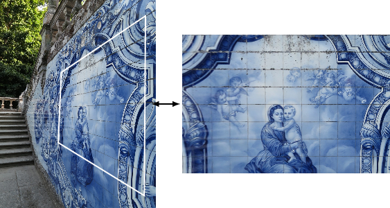
The applications involving homographic transformations are numerous. They will be discussed in detail in chapter 8 regarding the pin-hole camera, but in summary, such transformations allow for the removal of perspective from image planes, the projection of planes in perspective, and the association of points of planes observed from different viewpoints.

Un way to obtain perspective transformations is to relate points between the planes to be transformed and thereby determine the parameters of the homographic matrix (1.75), even in an over-dimensional manner, for example through the method of least squares. One way to derive the coefficients will be shown in equation (8.49). It should be noted that this transformation, which links points of planes between two perspective views, holds true only for the points of the considered planes: the homography relates points of planes to one another, but only those. Any point not belonging to the plane will be reprojected incorrectly.

It is easy to see that every homography is always invertible and the inverse of the transformation is also a homographic transformation:

$$\left( \mathbf{H}^{\Pi}_{ij} \right)^{-1} = \mathbf{H}^{\Pi}_{ji}$$ (1.79)

A possible form for the inverse of the homography (1.75) is

$$\begin{array}{l} u_i = \dfrac{(h_5 h_7 - h_4 h_8)u_j + (h_1... ...u_j + (h_0 h_7 - h_1 h_6) v_j + h_1 h_3 - h_4 h_0 } \end{array}$$ (1.80)

and, being known up to a multiplicative factor, no division has been used in deriving the parameters of the inverse transformation (unnormalized inverse homographic matrix).

It is worth noting that when the two planes related are parallel, then $h_{6}=0 \wedge h_{7}=0$, the homographic transformation reduces to an affine transformation represented by the classic equations

$$\begin{array}{l} u_j = h_0 u_i + h_1 v_i + h_2 \\ v_j = h_3 u_i + h_4 v_i + h_5 \end{array}$$ (1.81)

previously encountered.