Implicit 3D Modeling: RBFs and Signed Distance Fields (SDFs)

Implicit representations are not limited to radiance fields, however. The same principle of representing geometry through a continuous field can be used directly to describe a surface, independently of the rendering problem. A classic example is provided by Signed Distance Fields, which can also be constructed using radial basis functions.

While point clouds and polygonal meshes provide an explicit representation that is often fragmented or rigid, advanced geometric modeling frequently relies on implicit and continuous representations. One approach is to model the surface $\mathcal{S}$ as the zero level set of an implicit field:

$$\mathcal{S} = \left\{ \mathbf{x}\in\mathbb{R}^3 \mid f(\mathbf{x})=0 \right\}.$$ (10.122)

When the field $f(\mathbf{x})$ also represents the signed distance from the surface, it constitutes a Signed Distance Function (SDF), and in regular regions it ideally satisfies $\Vert\nabla f(\mathbf{x})\Vert=1$. One possible parameterization of the implicit field is obtained through a linear combination of Radial Basis Functions (RBFs) centered at the nodes $\mathbf{c}_i$:

$$f(\mathbf{x}) = \sum_{i=1}^{N} w_i \, \phi\left( \Vert\mathbf{x} - \mathbf{c}_i\Vert, R_i \right) + P(\mathbf{x})$$ (10.123)

Specifically:

• $\mathbf{c}_i = [c_{ix}, c_{iy}, c_{iz}]^T$ represents the position of the center of the $i$-th RBF.
• $w_i$ is the weight associated with the center.
• $R_i$ is the radius or support factor of the kernel, such as a cubic kernel $r^3$ or compactly supported functions such as Wendland functions.
• $P(\mathbf{x})$ is a low-degree polynomial that ensures the global stability of the field.

This approach can be used to reconstruct three-dimensional shapes from noisy point clouds, for example, those acquired using LiDAR. Given a measured point $\mathbf{y}_k$, the residual with respect to the implicit surface can be expressed directly as

$$r_k = f(\mathbf{y}_k).$$ (10.124)

The field parameters can then be determined through interpolation or optimization, depending on the formulation adopted, possibly using robust cost functions to reduce the influence of outliers.

Examples of RBF Kernels.

Depending on the desired geometric properties—whether to smooth the space globally or maintain efficient local support—different formulations of the radial kernel $\phi(r, R_i)$ (with $r = \Vert\mathbf {x} - \mathbf {c}_i\Vert$) are used:

• Global Cubic Kernel:
  

  $$\phi(r) = r^3 \quad (\text{oppure } r^5)$$ (10.125)

  
  
  This is one of the classic kernels for surface reconstruction. Since it is global, every center influences the entire space, ensuring very high regularity ($C^2$ or higher) but producing dense matrices that can become computationally expensive to solve as the number of centers increases.

• Gaussian Kernel:
  

  $$\phi(r, R_i) = \exp\left( -\frac{r^2}{2 R_i^2} \right)$$ (10.126)

  
  
  This kernel is widely used in machine learning and function approximation. The parameter $R_i$ acts directly as the standard deviation (width) of the Gaussian bell, determining how rapidly the influence of the center decays with distance.

• Wendland Compactly Supported Kernel:
  

  $$\phi(r, R_i) = \begin{cases} \left(1 - \frac{r}{R_i}\right)^... ...) & \text{se } r \le R_i \\ 0 & \text{se } r > R_i \end{cases}$$ (10.127)

  
  
  By becoming exactly zero beyond the threshold $R_i$, it ensures that each point in space is affected only by nearby centers; this makes the Jacobian matrix highly sparse and can improve computational efficiency even with a large number of centers.

• Multiquadratic Kernel:
  

  $$\phi(r, R_i) = \sqrt{r^2 + R_i^2}$$ (10.128)

  
  
  Characterized by linear growth at infinity, controlled by the scale parameter $R_i$, it is often used to interpolate sparse data when one wants to avoid the decay to zero typical of Gaussian kernels.

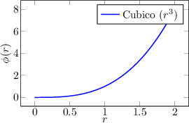
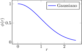
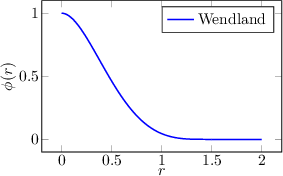
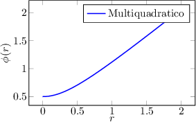
Figure 10.4: Behavior of the different radial basis function (RBF) kernels as a function of distance $r = \Vert\mathbf {x} - \mathbf {c}_i\Vert$.