SVM

LDA aims to maximize the statistical distance between classes but does not assess the actual margin of separation between them.

Figure 4.3: Separation hyperplane between two classes obtained through SVM. The points on the margin (dashed line) are the Support Vectors.

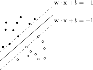SVM (CV95), like LDA, allows for the creation of a linear classifier based on a discriminant function in the same form as shown in equation (4.5). However, SVM goes further: the optimal hyperplane in $\mathbb{R}^{n}$ is generated in such a way as to "physically" separate (the decision boundary) the elements of the binary classification problem, aiming to maximize the separation margin between the classes. This reasoning greatly benefits the generalization of the classifier.

Let us therefore define the classification classes typical of a binary problem in the form $y_i = \{+1,-1\}$ and refer to the hyperplane given by formula (4.4).

Suppose there exist optimal parameters $(\mathbf{w}_0,b_0)$ that satisfy the constraint

$$\begin{array}{ll} \mathbf{x}_i \cdot \mathbf{w}_0 + b_0 \ge... ...athbf{w}_0 + b_0 \leq -1 & \text{per } y_i = -1 \\ \end{array}$$ (4.16)

or, in a more compact form:

$$y_i ( \mathbf{x}_i \cdot \mathbf{w}_0 + b_0 ) - 1 \geq 0$$ (4.17)

for every $(y_i, \mathbf{x}_i)$ samples provided during the training phase.

It can be assumed that for each of the categories, there exists one or more vectors $\mathbf{x}_i$ where the inequalities (4.17) become equalities. These elements, referred to as Support Vectors, are the most extreme points of the distribution, and their distance represents the measure of the separation margin between the two categories.

The distance $\rho$ point-plane (see eq.(1.52)) is given by

$$\rho = \frac{ \Vert \mathbf{w} \cdot \mathbf{x} + b \Vert } { \Vert \mathbf{w} \Vert }$$ (4.18)

Given two points of opposite classes that satisfy the equality (4.17), the margin can be derived from the equation (4.18), and it is equal to

$$\rho = \frac{2}{\Vert \mathbf{w}_0 \Vert}$$ (4.19)

To maximize the margin $\rho$ of equation (4.19), one must minimize its inverse, that is,

$$\min_{\mathbf{w},b} \frac{1}{2} \Vert \mathbf{w} \Vert^2$$ (4.20)

under the series of constraints expressed by the inequality (4.17). This is what is referred to as the standard primal optimization problem of the SVM.

This class of problems (minimization with constraints such as inequalities or primal optimization problem) is solved using the Karush-Kuhn-Tucker approach, which is the method of Lagrange multipliers generalized to inequalities. Through the KKT conditions, the Lagrangian function is obtained:

$$\mathcal{L}(\mathbf{w}, b, \boldsymbol\alpha) = \frac{1}{2}... ...i \left( y_i ( \mathbf{x}_i \cdot \mathbf{w} + b ) - 1 \right)$$ (4.21)

to be minimized in $\mathbf{w}$ and $b$ and maximized in $\boldsymbol\alpha$. The weights $\alpha_i \geq 0$ are the Lagrange multipliers.

From the nullification of the partial derivatives, we obtain:

$$\frac{\partial \mathcal{L} }{\partial b} = 0 \rightarrow \sum y_i \alpha_i = 0$$ (4.22)

$$\frac{\partial \mathcal{L}}{\partial \mathbf{w}} = 0 \rightarrow \mathbf{w} = \sum \alpha_i y_i \mathbf{x}_i$$ (4.23)

By substituting these results (the primal variables) into the Lagrangian (4.21), it becomes a function of the multipliers only, the dual, from which the Wolfe dual form is derived:

$$\Psi (\boldsymbol\alpha) = \sum \alpha_i -\frac{1}{2} \sum_... ...um_j \alpha_i \alpha_j y_i y_j \mathbf{x}_i \cdot \mathbf{x}_j$$ (4.24)

under the constraints $\alpha_i \ge 0$ and $\sum \alpha_i y_i = 0$. The maximum of the function $\Psi$ evaluated over $\boldsymbol\alpha$ corresponds to the $\alpha_i$ associated with each training vector $\mathbf{x}_i$. This maximum allows us to find the solution to the original problem.

In this relationship, the KKT conditions are valid, among which the constraint known as Complementary slackness is of considerable importance.

$$\alpha_i \left( y_i ( \mathbf{x}_i \cdot \mathbf{w} + b ) - 1 \right) = 0$$ (4.25)

This constraint states that the maximum of the Lagrangian is either on the boundary of the constraint ( $\alpha_i\neq 0$) or is a local minimum ($\alpha_i = 0$). As a consequence, only the $\alpha_i$ on the boundary are non-zero and contribute to the solution: all other training samples are, in fact, irrelevant. These vectors, associated with the $\alpha_i > 0$, are the Support Vectors.

By solving the quadratic problem (4.24), under the constraint (4.22) and $\alpha_i \geq 0$, the weights that exhibit $\alpha_i\neq 0$ will be the Support Vectors. These weights, when substituted into equations (4.23) and (4.25), will lead to the derivation of the maximum margin hyperplane.

The most commonly used method to solve this QP problem is the Sequential Minimal Optimization (SMO). For a comprehensive discussion of the topics related to SVM, one can refer to (SS02).