Sigma-Point Kalman Filter

An alternative to the extended Kalman filter for nonlinear systems is the Sigma-Point Kalman Filter. According to results reported by various experiments, for nonlinear functions $f$ and $h$, the Sigma Point Kalman Filter (SPKF) tends to provide better performance than the EKF: the statistically linearized error propagation (SPKF) is generally better than propagation based on a Taylor-series expansion (EKF).

Not only the state, but also the various points around the mean (the sigma points) are propagated through the functions that compose the Kalman state update and observation. The advantage of the SPKF is that it does not require computing Jacobians and normally provides a better estimate of the process mean and variance.

The Unscented Kalman filter (Unscented Kalman filter) is one of several versions of the Sigma-Point Kalman Filter. In this case, the uncertainty-propagation theory discussed in Section 2.6.2 is used to estimate the mean and covariance of the a priori state and observation error.

The Unscented filter can also handle the case in which noise enters the system non-additively. To generalize the non-additive-noise case, and maintain the same syntax discussed in Section 2.6.2, we define a variable called the augmented state $\mathbf{x}^{a} \in \mathbb{R}^{n^{a}}$ with $n^{a}=n+q$, consisting of the state $\mathbf{x}\in\mathbb{R}^{n}$ and the zero-mean process noise $w$, so as to use the function

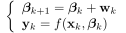$${\bm{\mathcal{X}}}^{-} = f(\mathbf{x}^{a}_{k-1}, \mathbf{u}_{k} )$$ (3.33)

for the state update, allowing the contribution of the process noise to be taken into account nonlinearly and non-additively. Similarly, we define the augmented covariance matrix as:

$$\mathbf{P}_{\mathbf{x}}^{a} = \begin{bmatrix} \mathbf{P}_{\mathbf{x}} & 0 \\ 0 & \mathbf{Q} \end{bmatrix}$$ (3.34)

When the process noise is additive, the system becomes similar to the linear Kalman system, with the form

$$\mathbf{P}^{-}_{k} = \sum_{i=0}^{2n} w^{c}_i ({\bm{\mathcal... ...{i} - \bar{{\bm{\mathcal{X}}}}^{-}_{i} )^{\top} + \mathbf{Q}_k$$ (3.35)

From the sigma points ${\bm{\mathcal{X}}}^{-}_{i}$, projected through $f$ and representing the a priori state distribution, it is possible to generate additional sigma points in order to estimate the a priori observation:

$${\bm{\mathcal{Z}}}_i = h({\bm{\mathcal{X}}}^{-}_{i})$$ (3.36)

which can be used to calculate the most probable observation value $\hat{\mathbf{z}}$ by weighting the results ${\bm{\mathcal{Z}}}_i$ with the weights associated with the sigma points, as in equation (2.49). Here too, observation noise can be included as an augmented state or, if assumed to be additive and independent, added to the covariance matrix.

Knowing the sigma points ${\bm{\mathcal{X}}}^{-}_{i}$ and ${\bm{\mathcal{Z}}}_i$, it is straightforward to obtain the covariance $\cov (\bm{\mathcal{Z}})$ and the cross-covariance $\cov (\bm{\mathcal{X}},\bm{\mathcal{Z}})$ by generalizing equation (2.49):

$$\cov \left( \bm{\mathcal{X}},\bm{\mathcal{Z}}\right) \appro... ...bar{\mathbf{x}})(\bm{\mathcal{Z}}_i - \bar{\mathbf{z}})^{\top}$$ (3.37)

Given the covariance $\cov (\bm{\mathcal{Z}})$ and the cross-covariance $\cov (\bm{\mathcal{X}},\bm{\mathcal{Z}})$, the sigma-point Kalman gain is exactly the same as that given by equation (3.22), and the covariance update $\mathbf{P}_{k}$ follows equation (3.23).