Kalman Filter

The Kalman filter (WB95) estimates, in the presence of disturbances, the inaccessible internal state $\mathbf{x}\in\mathbb{R}^{n}$ of a discrete-time system whose model is completely known. In fact, the Kalman filter is the optimal recursive estimator: if the problem noise is Gaussian, the Kalman filter provides the minimum-mean-square estimate of the system's internal state.

For historical reasons, the Kalman filter properly refers only to filtering a system in which state transition and observation are linear functions of the current state.

According to linear systems theory, the dynamics of a continuous-time “linear” system are represented by a differential equation of the form

$$\dot{\mathbf{x}} = \mathbf{A}(t) \mathbf{x}(t) + \mathbf{B} \mathbf{u}(t) + \mathbf{w}(t)$$ (3.11)

the state update equation, associated with an indirect observation of this state through a linear system:

$$\mathbf{z}(t) = \mathbf{H}(t) \mathbf{x}(t) + \mathbf{v}(t)$$ (3.12)

where $\mathbf{z} \in \mathbf{R}^{m}$ is the observable.

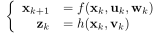
The discrete-time Kalman filter is useful for real systems in which the world is sampled at discrete intervals, transforming the continuous-time linear system into a linear system of the form

$$\left\{ \begin{array}{l} \mathbf{x}_{k+1} = \mathbf{A}_{k} ... ...mathbf{H}_k \mathbf{x}_{k} + \mathbf{v}_{k} \end{array}\right.$$ (3.13)

If the system evolves according to this model, it is called a Linear-Gaussian State Space Model or Linear Dynamic System. If the matrix values are independent of time, the model is called stationary.

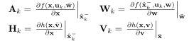The variables $w_{k}$ and $v_{k}$ represent process and observation noise, respectively, with zero mean $\bar{w_k}=\bar{v_k}=0$ and known covariance matrices $\mathbf{Q}$ and $\mathbf{R}$, respectively (white Gaussian noise is assumed). $\mathbf{A}$ is a $n \times n$ state-transition matrix, $\mathbf{B}$ is a $n \times l$ matrix that connects the optional control input $\mathbf{u} \in \mathbb{R}^{l}$ to the state $\mathbf {x}$, and finally $\mathbf{H}$ is a $m\times n$ matrix that connects the state to the measurement $\mathbf{z}_{k}$. All these matrices, which represent the system model, must be known with absolute precision; otherwise, systematic errors are introduced.

The Kalman filter is a recursive state estimator and requires, at each iteration, knowledge of the state estimated at the previous step $\hat{\mathbf{x}}_{k-1}$ and the current observation $\mathbf{z}_k$, which is an indirect observation of the system state.

Let $\hat{\mathbf{x}}^{-}_{k}$ be the a priori estimate of the system state, based on the estimate obtained at time $k-1$ and on the system dynamics, and let $\hat{\mathbf{x} }_{k}$ be the a posteriori state estimate based on the observation $\mathbf{z}_k$. These definitions allow the a priori and a posteriori estimation errors to be defined as

$$\begin{array}{l} \mathbf{e}^{-}_{k} = \mathbf{x}_k - \hat{\... ...bf{e}_{k} = \mathbf{x}_k - \hat{\mathbf{x}}_{k} \\ \end{array}$$ (3.14)

These errors can be associated with

$$\begin{array}{l} \mathbf{P}^{-}_k = \E[\mathbf{e}^{-}_k {\m... ...\mathbf{P}_k = \E[\mathbf{e}_k \mathbf{e}^{\top}_k] \end{array}$$ (3.15)

the a priori and a posteriori error covariance matrices, respectively.

The objective of the Kalman filter is to minimize the a posteriori error covariance $\mathbf{P}_k$ and provide a method for obtaining the estimate of $\hat{\mathbf{x} }_{k}$ given the a priori estimate $\hat{\mathbf{x}}^{-}_{k}$ and the observation $\mathbf{z}_k$.

The Kalman filter provides an a posteriori state estimate through a linear combination of the previous state estimate and the observation error:

$$\hat{\mathbf{x}}_{k} = \hat{\mathbf{x}}^{-}_{k} + \mathbf{K}_k( \mathbf{z}_k - \mathbf{H}_k \hat{\mathbf{x} }^{-}_{k})$$ (3.16)

thus reducing the estimation problem to finding the gain factor $\mathbf{K}_k$ (blending factor). The difference $\mathbf{z}_k - \mathbf{H}_k \hat{\mathbf{x} }^{-}_{k}$ is called the residual, or innovation, and represents the discrepancy between the predicted observation and the actual observation. Note that the metric used to calculate the residual may depend on the particular characteristics of the problem. The Kalman filter is normally presented in two phases: time update (prediction phase) and measurement update (observation phase).

In the first phase, the a priori estimate of both $\hat{\mathbf{x}}_k$ and the covariance $\mathbf{P}_{k}$ is obtained. The a priori estimate $\hat{\mathbf{x}}^{-}_{k}$ follows from knowledge of the system dynamics (3.13):

$$\hat{\mathbf{x}}^{-}_{k} = \mathbf{A}_{k-1} \hat{\mathbf{x}}_{k-1} + \mathbf{B}_{k-1} \mathbf{u}_{k-1}$$ (3.17)

and the a priori estimate of the error covariance is updated similarly:

$$\mathbf{P}^{-}_{k} = \mathbf{A}_{k-1} \mathbf{P}_{k-1} \mathbf{A}_{k-1}^{\top} + \mathbf{Q}_{k-1}.$$ (3.18)

These are the best a priori estimates of the state and covariance at time $k$ that can be obtained before observing the system.

In the second phase, the gain is computed:

$$\mathbf{K}_k = \mathbf{P}^{-}_{k} \mathbf{H}_k^{\top} \left... ...hbf{P}^{-}_{k} \mathbf{H}_k^{\top} + \mathbf{R}_k \right)^{-1}$$ (3.19)

this gain minimizes the a posteriori covariance and is used to update the a posteriori state through equation (3.16).

Using this value for the gain $\mathbf{K}$, the a posteriori estimate of the covariance matrix becomes

$$\mathbf{P}_{k} = (\mathbf{I} - \mathbf{K}_k \mathbf{H}_k) \mathbf{P}^{-}_{k}$$ (3.20)

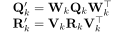
To unify the different variants of Kalman filters, these equations can be rewritten using the variance-covariance matrices

$$\begin{array}{l} \cov (x_k, z_k) = \mathbf{P}^{-}_{k} \mat... ...mathbf{H}_k \mathbf{P}^{-}_{k} \mathbf{H}_k^{\top} \end{array}$$ (3.21)

so that equation (3.19) can be written as

$$\mathbf{K}_k = \cov (x_k, z_k) \left( \cov (z_k) + \mathbf{R}_k \right)^{-1}$$ (3.22)

and, substituting the covariances (3.21) into (3.20), we obtain

$$\mathbf{P}_{k} = \mathbf{P}^{-}_{k} - \mathbf{K}_k \cov (x_k, z_k)^{\top}$$ (3.23)

As can readily be seen, the covariance matrix and the Kalman gain depend neither on the state nor on the observations, and even less on the residual; instead, they have an independent history.

Kalman filtering nevertheless requires an initial value for the state variable and the covariance matrix: the initial state value must be as close as possible to the true value, and the degree of similarity to this value must be encoded in the initial covariance matrix.