Grid-based Methods

Grid-based approaches are particularly well suited to problems in which the state assumes only a limited number of discrete values (and are therefore called discrete filters), while they provide an approximate estimate when the state is continuous (histogram filters) and is discretized through spatial quantization. Each element of the grid (or histogram) is assigned the probability that the state actually lies in that particular cell. Bayesian filter theory (and therefore multimodal distributions and strongly nonlinear systems) is used directly, but is restricted to the discrete points at which the state can exist.

Suppose that $m$ points are used to represent the state $\mathbf{x}\in\mathbb{R}^{n}$. If the original state is continuous, this is clearly an approximation, and it is preferable that $m \gg n$. At each iteration $k$, there are therefore 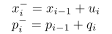$\mathbf{x}_{i,k} \in \mathbb{R}^{n}$ with $i=1,\ldots,m$ possible states, associated with a probability distribution $p_{i,k}$ that evolves over time according to the system dynamics.

The equations introduced above apply, namely, the a priori estimate:

$$p^{-}_{i,k} = \sum_{j=1}^{m} p(x_{i,k} \vert x_{j,k-1}) p^{+}_{j,k-1}= \sum_{j=1}^{m} f_{i,j} p^{+}_{j,k-1} \quad \forall i$$ (3.9)

and the state update equation a posteriori of observation $z_k$:

$$p^{+}_{i,k} = c_k p(z_k \vert x_{i,k}) p^{-}_{i,k} \quad \forall i$$ (3.10)

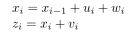where $c_k$ is again the normalization factor such that $\sum p^{+}_i = 1$.

Grid-based methods therefore make it possible to apply recursive Bayesian theory directly.