


Next: Corresponding points in alternative Up: Multi-Camera Vision Previous: Chirality and reconstruction from
As seen in section 10.3.1, triangulating noisy points leads to non-intersecting lines whose intersection does not minimize the residual in image coordinates (for example, under the Euclidean-distance metric). We also saw that the best estimate of the noise-free points minimizes the quantity in equation 10.72 subject to the epipolar constraint 10.73. So far, however, given the Essential/Fundamental Matrix, this minimization has required the three-dimensional point as an auxiliary variable and an (iterative) optimization technique initialized, for example, by exploiting the triangulation of noisy points using skew lines.
A global nonlinear technique makes it possible to obtain the optimal triangulation (the estimate of the image points) through a polynomial method (HS97) that requires finding the roots of a sixth-degree polynomial.
As discussed more clearly in (Lin10), optimal triangulation can be viewed as the following minimization problem:
 |
(10.90) |
 |
(10.91) |
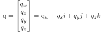 and
and
 have been defined, and the matrix
 |
(10.92) |
 are the estimates of the noise-free points, whereas
 are the observed points.
This constrained minimization problem can be solved using Lagrange multipliers:
 |
(10.93) |
 |
(10.94) |
 ).
These constraints can be parameterized as a function of an auxiliary variable, from which the well-known sixth-degree equation is obtained.
This approach is exactly the same whether image points and the Fundamental Matrix or camera points and the Essential Matrix are used.
).
These constraints can be parameterized as a function of an auxiliary variable, from which the well-known sixth-degree equation is obtained.
This approach is exactly the same whether image points and the Fundamental Matrix or camera points and the Essential Matrix are used.
Also in (Lin10), suboptimal iterative techniques with low computational cost are presented, in which the epipolar constraint is nevertheless satisfied at every iteration.
Once the noise-free image points have been obtained, the three-dimensional point can be recovered using any triangulation technique (the skew-line method of section 1.6.6 or the DLT of section 10.3.1).
An alternative formulation (KK95), given two corresponding points expressed in camera coordinates
 and
and
 , is that the three-dimensional point formed by the intersection of the optical rays is
 |
(10.95) |
 .
.