Förstner-Harris

The Förstner-Harris algorithm (FG87,HS88) has been explicitly designed to achieve high geometric stability. It defines characteristic points as those points that exhibit a local maximum when compared to the least squares of their translated version. This algorithm has been highly successful because it enables the identification of variations in image intensity in the vicinity of a point by utilizing the autocorrelation matrix of the first derivatives of the image.

Let the gradient images be defined (these can be generated by a differential operator, such as Sobel, Prewitt, or Roberts) as $I_x(x,y)$ and $I_y(x,y)$, representing the horizontal gradient and the vertical gradient of the image to be analyzed, respectively.

From these two images, it is possible to calculate a function $\mathbf{C}(x,y)$, representing the covariance matrix (autocorrelation) of the gradient images in the vicinity of $(x,y)$, defined as It seems that you have included a placeholder for a mathematical block, but there is no content provided for translation. Please provide the specific text or equations that you would like to have translated from Italian to English, and I will be happy to assist you. with $\boldsymbol\delta \in \Omega$ around $(x,y)$ and $w(\boldsymbol\delta)$ an optional kernel, typically a Gaussian centered at $(x,y)$, to allow for differential weighting of the points in the vicinity, or a constant window on $\Omega$. Originally, $w(\boldsymbol\delta)$ were very small filters, but as computational power has increased, larger Gaussian kernels have been adopted.

In fact, Harris employs two convolution filters: a derivative filter to compute the derived images and an integral filter to calculate the elements of the matrix. The dimensions of these filters and the use of a Gaussian filter to weight the points refer to the discussion in the following section regarding the scale of feature detection.

The matrix $\mathbf{C}$ is the second-order moment matrix. To identify characteristic points, one can analyze the eigenvalues $\lambda_0$ and $\lambda_1$ of the matrix $\mathbf{C}$ (for a more in-depth discussion, refer to section 2.10.1). The eigenvalues of the autocorrelation matrix $\mathbf{C}$ allow for the characterization of the type of image contained within the window around the given point.

If there are two very high eigenvalues, the point is a corner; if there is only one high eigenvalue, it is an edge; otherwise, it is a reasonably flat area, represented as a function like

$$C = \min( \lambda_0, \lambda_1 )$$ (5.3)

where the local maxima correspond to the corners identified by the Shi-Tomasi algorithm (ST94).

For a matrix $2 \times 2$, the eigenvalues are obtained as solutions of the quadratic characteristic polynomial

$$p(x) = x^2 - \trace (\mathbf{C}) x + \det(\mathbf{C})$$ (5.4)

.

Harris, to avoid explicitly calculating the eigenvalues of $\mathbf{C}$, introduces an operator $H(x,y)$ defined as

$$H(x,y) = \det(\mathbf{C}) - \alpha \trace (\mathbf{C})^{2}$$ (5.5)

where $\alpha$ is a parameter that lies between $0$ and $0.25$ and is typically set to $0.04$.

Figure 5.1: Response in the eigenvalue plane provided by the Harris equation at different threshold values, with $\alpha =0.04$ set. The area of interest is very similar to that provided by the Shi-Tomasi method but without the need to explicitly compute the eigenvalues.

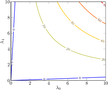According to Harris, the point $(x,y)$ is a characteristic point (corner) if $H(x,y) > H_{thr}$, with $H_{thr}$ being a threshold to be defined. The parameter $\alpha$ regulates the sensitivity of the feature detector. Qualitatively, increasing $\alpha$ removes edges, while increasing $H_{thr}$ removes flat areas (figure 5.1).