AdaBoost and Its Variants

Figure 5.7: Comparison of loss functions: 0/1 loss, logistic, exponential, and quadratic

The Boosting problem can be generalized and viewed as a problem in which predictors $f_t(\mathbf{x})$ must be found that minimize the global cost function:

$$\sum_{i=1}^{m} \phi \left( y_i \left( f_1(\mathbf{x}_i) + \ldots + f_n(\mathbf{x}_i) \right) \right)$$ (5.92)

where $\phi \in \mathcal{C}^1$ is a convex, non-increasing function of $\lim_{z \to \infty} \phi(z)=0$.

From an analytical perspective, AdaBoost is an example of a coordinate-wise gradient-descent optimizer that minimizes the potential function $\phi(z)=e^{-z}$, optimizing one coefficient $\alpha_t$ at a time (LS10), as shown by Equation (5.81).

The following is a non-exhaustive list of AdaBoost variants that highlights some of the distinctive features of this technique:

AdaBoost with Abstention

AdaBoost can also be extended to classifiers with abstention, for which the possible outputs are $h_j(x_i) \in \{-1,0,+1\}$. Extending Definition (5.84), for simplicity let $W_{-}$ denote failures, $W_{0}$ abstentions, and $W_{+}$ successes of classifier $h_t$.

In this case as well, $Z_t$ attains its minimum with the same value $\alpha_t$ as in the case without abstention; see (5.90), and with this choice $Z_t$ would be

$$Z_t = W_0 + 2 \sqrt{ W_{-} W_{+}}$$ (5.93)

However, Freund and Shapire proposed a more conservative choice of $\alpha_t$:

$$\alpha_t = \frac{1}{2} \log \left( \frac{W_{+} + 1/2 W_0}{W_{-} + 1/2 W_0} \right)$$ (5.94)

which makes it possible to establish an upper bound on $Z_t$.

Real AdaBoost

Real AdaBoost generalizes the preceding case and, above all, generalizes the same extended additive model (FHT00). Instead of using dichotomous hypotheses $h_t(x)$ and assigning them a weight $\alpha_t$, it directly seeks the feature $f_t(x)$ that minimizes Equation (5.81).

Real AdaBoost allows weak classifiers to provide the probability distribution $p_t(x) = P[y=1 \vert x, w^{(t)} ] \in [0,1]$, namely the probability that class $y$ is actually $+1$ given the observation of feature $x$.

Given a probability distribution $p_t(x)$, the feature $f_t(x)$ that minimizes Equation (5.81) is

$$f_t(x) = \frac{1}{2} \log \frac{ P [y=+1 \vert x, w^{(t)} ] ... ...vert x, w^{(t)} ] } = \frac{1}{2} \log \frac{p_t(x)}{1-p_t(x)}$$ (5.95)

This result is equal to half of the logistic transformation. Since the objective remains to minimize the exponential cost function, the weight update is still the one given by Equation (5.87). Both Discrete and Real AdaBoost, by choosing a weak classifier that satisfies Equation 5.95, ensure that AdaBoost converges asymptotically to

$$\lim_{T \to \infty} F_T(x) = \frac{1}{2} \log \frac{P[y=+1\vert x]}{P[y=-1\vert x]}$$ (5.96)

demonstrating that the AdaBoost algorithm is an iterative procedure that combines several weak classifiers to approximate a Bayesian classifier.

Real AdaBoost can also be used with a discrete classifier such as the Decision Stump. By directly applying Equation (5.95) to the two possible output states of the Decision Stump (the minimum of $Z_t$ can nevertheless be obtained easily algebraically), the classifier responses must take the values

$$f(x) = \left\{ \begin{array}{ll} \frac{1}{2} \log \frac{W_... ...\log \frac{W_{FN}}{W_{TN}} & x \leq \theta \end{array}\right.$$ (5.97)

with values $W_{*}$, the sums of the weights associated with False Positives (FPs), False Negatives (FNs), True Positives (TPs), and True Negatives (TNs). With this choice of values, $Z_t$ assumes the notable value

$$Z_t = 2 \left( \sqrt{W_{TP}W_{FP}} + \sqrt{W_{FN}W_{TN}} \right)$$ (5.98)

the metric to be used to select the best feature $x$ and threshold $\theta$.

Gentle AdaBoost

The weights associated with outliers in Real AdaBoost can become very large because of the logarithm in the equation. In this case, it is desirable to make the regression more “gentle.”

Gentle AdaBoost further generalizes the concept of Ensemble Learning to an additive model (FHT00) by using a regression with steps typical of Newton methods:

$$F_{T+1}(x) = F_T(x) + f_t(x) = F_T(x) + \E_{w^{(t)}} [ y \vert x ]$$ (5.99)

The hypothesis $f_t(x)$ to be added to the additive model at iteration $t$ is selected from all possible hypotheses $f_k$ as the one that optimizes a weighted least-squares regression:

$$f_t = \argmin_{f_k} \sum_i w_i (y_i - f_k(x_i))^2$$ (5.100)

but at each iteration the AdaBoost weight update is used (5.87), namely the exponential cost function. Gentle AdaBoost can also be used with the Decision Stump. In this case, the minimum of (5.100) in the decision algorithm takes the notable form

$$f(x) = \left\{ \begin{array}{ll} \frac{W_{TP} - W_{FP} }{ ... ..._{TN} }{ W_{TN} + W_{FN} } & x \leq \theta \end{array}\right.$$ (5.101)

LogitBoost

For historical reasons, AdaBoost does not explicitly exhibit a statistical formalism. The first observation is that the response of the AdaBoost classifier is not a probability, since it is not bounded between $[0,1]$. In addition to this problem, which is partially resolved by Real AdaBoost, minimizing the loss function (5.80) does not appear to be a statistical approach, unlike maximizing the likelihood. Nevertheless, it can be shown that the AdaBoost cost function maximizes a function very similar to the Bernoulli log-likelihood.

For these reasons, AdaBoost can be extended to logistic regression theory, described in Section 5.4.

Additive logistic regression takes the form

$$\log \frac{P[y=+1\vert x]}{P[y=-1\vert x]} = F_T(x) = \sum_{t=1}^{T} f_t(x)$$ (5.102)

which is an interesting expression when compared with the AdaBoost expression in Equation (5.96). Inverting Equation (5.102) yields the logistic relationship

$$p(x) = P[y=+1\vert x] = \frac{e^{F_T(x)} }{1 + e^{F_T(x)} } = \frac{1}{1+e^{-F_T(x)}}$$ (5.103)

which associates a probability estimate with the additive model $F(x)$.

The problem is to find a suitable loss function for this representation, that is, to identify an AdaBoost variant that exactly maximizes the Bernoulli log-likelihood (FHT00).

Maximizing the likelihood of (5.103) is equivalent to minimizing the log-loss

$$\sum_{t=1}^{T} \log \left( 1 + \exp ( -y_i F_T(x_i) ) \right)$$ (5.104)

LogitBoost was the first method to extend AdaBoost to the logistic optimization problem for a function $F_T(x)$ under the cost function $\phi(z)=\log \left(1 + e^{-z} \right)$, maximizing the Bernoulli log-likelihood using Newton-type iterations.

The weights associated with each sample follow directly from the probability distribution

$$\begin{array}{l} z_i = \frac{y_i^{*} - p(x_i)}{p(x_i) (1 - p(x_i) )} \\ w_i = \frac{ p(x_i) }{1 - p(x_i) } \end{array}$$ (5.105)

where $y^{*}=\left\{0,1\right\}$, and the hypothesis $f_t(x)$ is selected as the least-squares regression of $z_i$ on $x_i$ using the weights $w_i$. The future estimate of $p(x_i)$ follows directly from Equation (5.103).

Asymmetric AdaBoost

Asymmetric AdaBoost introduces a variant of the weight-update rule (VJ01). The problem with AdaBoost is that it does not provide direct control over the weight assigned to classification errors in the different classes, nor does it explicitly minimize the number of false positives, but only the classification error. The Asymmetric AdaBoost variants instead modify, at each iteration $t$, the weights associated with positive and negative samples by cost factors $c^{(t)}_{+}$ and $c^{(t)}_{-}$, respectively.

Cascade

Regardless of whether Cascade classifiers (VJ02) are used, the weights are modified by a factor $\beta_t = \epsilon_t/(1-\epsilon_t) = W_{-}/W_{+}$ only in the case of correct classification; otherwise, the weights remain unchanged. The weight associated with a classifier is assigned as $\alpha_t = - \log \beta_t$, twice the weight assigned by AdaBoost.M1.

MAdaBoost

The MAdaBoost algorithm uses a different weight update to reduce the contribution of outliers (or overly complex examples) during training. The maximum weight $w^{(t)}_i$ that a sample can attain is upper-bounded by $w^{(0)}_i$, the value assigned to the weight at the beginning of the algorithm.

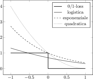
This behavior can be represented by a cost function of the form

$$\phi(z)=\left\{\begin{array}{ll} 1-z & z \leq 0 \\ e^{-z} & z > 0 \\ \end{array}\right.$$ (5.106)