ADAptive BOOSTing

One of the Ensemble classifiers that has attracted the greatest interest from researchers in recent years is undoubtedly AdaBoost (FS95). The basic idea behind AdaBoost is to construct a list of classifiers by iteratively assigning a weight to each new classifier according to its ability to recognize samples that were not correctly identified by the other classifiers already involved in training. All these classifiers vote with their assigned weights, and the final decision is made by majority vote.

Boosting techniques make it possible to generate a classifier in the form of an additive model:

$$F_T(\mathbf{x}) = f_1(\mathbf{x}) + f_2(\mathbf{x}) + \ldots + f_T(\mathbf{x}) = \sum_{t=1}^{T} f_t(\mathbf{x})$$ (5.79)

with $f_1,\ldots,f_T$ individual classifiers.

Let us examine the binary classification case, and let $S=(\mathbf{x}_1,y_1) \ldots (\mathbf{x}_m, y_m) \in (\mathbb{X} \times \{-1,1\} )$ be the set of $m$ samples available for training.

A fairly common choice when fitting models is to use least-squares regression (an optimal metric in the presence of Gaussian noise, for example) to obtain the additive model $F_T(\mathbf{x})$, by minimizing the quantity $\sum \left( y_i - F_T(\mathbf{x}_i) \right)^2$. However, numerous experiments have shown that the quadratic cost function is not the optimal choice for classification problems.

The AdaBoost approach instead suggests that the combination of all these classifiers should minimize a different, better cost function, namely the exponential loss:

$$\min_{F} \sum_{i=1}^{m} e^{-y_i F(\mathbf{x}_i)}$$ (5.80)

As discussed in Section 5.6, this function corresponds to the exponential loss. The objective of AdaBoost can therefore be interpreted as minimizing the empirical risk with respect to this loss function. The algorithm assigns a very high penalty to samples with a negative margin, progressively focusing training on the examples that are more difficult to classify.

Since global minimization of the function (5.80) is usually impossible, two approaches can be followed:

• optimizing one classifier at a time cyclically until a stable situation is reached (generalized backfitting algorithm);
• adding one classifier at a time to the additive model (“greedy” forward stepwise approach)

AdaBoost addresses the classification problem using the second approach.

Under these assumptions, the objective of the training process is reduced to finding an additional classifier $f(\mathbf{x})$ that minimizes, at each step, the quantity

$$f_{T+1} = \argmin_{f} \sum_{i=1}^{m} e^{-y_i \left( F_T(\mat... ...} = \argmin_{f} \sum_{i=1}^{m} w_i e^{-y_i f(\mathbf{x}_i)}$$ (5.81)

where $w_i = e^{-y_i F_T(\mathbf{x}_i) }$ has been defined and the properties of the exponential function have been used.

AdaBoost is a technique that meets all these requirements.

Suppose, therefore, that $\mathcal{H}=\{h_1, \ldots, h_T\}$ binary classifiers are available, each of which, by evaluating feature $\mathbf{x}_i$, with $1 \leq i \leq m$, returns an opinion $y_i=\{-1,+1\}$.

Let the function $F_T(\mathbf{x};\boldsymbol\alpha)$, defined as

$$F_T(\mathbf{x};\alpha_1, \ldots, \alpha_T) = \sum_{t=1}^{T} \alpha_t h_t(\mathbf{x})$$ (5.82)

be a function whose sign represents the classification hypothesis and whose magnitude reflects the quality of the prediction. The model in Equation (5.82) is called the Extended Additive Model or Adaptive Basis-Function Model.

The objective is to obtain a strong classifier $H(\mathbf{x}_i)$ as a weighted linear sum of the classifiers $h_t$, whose sign determines the overall hypothesis:

$$H(\mathbf{x}_i) = \sgn \left( \sum^{T}_{t=1} \alpha_t h_t(\mathbf{x}_i) \right) = \sgn F_T(\mathbf{x}_i;\boldsymbol\alpha)$$ (5.83)

This is a majority vote: the hypothesis receiving the most votes is selected as the winner, with each classifier having a different weight $\alpha_t$. The constants $\alpha_t$—the weights assigned to each classifier—are precisely the result produced by this training technique.

To assign a vote to a classifier, each input sample $x_i$ must be assigned a weight $w_i$: the higher the weight, the more incorrectly the sample has been classified up to that point in training, whereas the lower the weight, the more correctly it has been classified. At the first iteration, all weights are set equal to $w_i^{(0)}=1/m$, so as to obtain an exact statistical distribution. Variants such as Asymmetric AdaBoost assign different weights to the different classes involved.

Let $u_i=y_i h_t(\mathbf{x}_i)$ be the function expressing the success ($+1$) or failure ($-1$) of classifier $h_t$ when evaluating sample $x_i$. Given the weights associated with each sample, for each classifier it is possible to calculate $W_{-1}$, the sum of the weights associated with failures, and $W_{+1}$, the sum of the weights associated with correct classifications, that is, by defining $u_i$, in compact form:

$$W_b = \sum_{ u_i = b } w_i$$ (5.84)

where $b=+1$ denotes success and $b=-1$ failure.

Let $\epsilon_t$ be the error measure of classifier $h_t$, calculated as

$$\epsilon_t = \sum_{y_i \neq h_t(i) } w_i^{(t)} = \sum_{u_i=-1} w_i^{(t)} = W_{-}$$ (5.85)

the sum of the weights associated only with incorrectly classified samples, and let

$$r_t = W_{+}-W_{-} = \sum_{i=1}^{m} w^{(t)}_i u_i$$ (5.86)

be the weighted average, using the weights $w_i$, of the classification performance $u_i$.

The iterations of the AdaBoost algorithm are as follows:

1. an Oracle provides a classifier $h_t$ (the choice is effectively left to the user, who attempts to select the classifier that minimizes the error $\epsilon_t$, although it is not required to be the best one);
2. the error $\epsilon_t$ produced by classifier $h_t$ on the input samples is calculated. When it is not possible to find a classifier for which $\epsilon_t > 1/2$, training cannot continue and must therefore be terminated;
3. given the error, a weight $\alpha_t$ is assigned to classifier $h_t$, calculated as described below;
4. for each sample $x_i$, the associated distribution $w_i^{(t+1)}$ is updated using the function
   

   $$w_i^{(t+1)} = \frac{1}{Z_t} w_i^{(t)} e^{ - \alpha_t u_i } = \frac{1}{Z_t} w_i^{(t)} e^{ - y_i f_t (\mathbf{x}_i) }$$ (5.87)

   
   
   The weight associated with samples that were classified correctly is decreased by an amount proportional to $e^{-\alpha_t}$, whereas the weight of incorrectly classified samples is increased by $e^{\alpha_t}$. $Z_t$ is a normalization factor chosen so that $\sum w_i^{(t)}=1$, but it also has an important meaning, as explained immediately below.

The normalization parameter $Z_t$ is

$$Z_t = \sum_{i=1}^{m} w_i^{(t)} e^{ - \alpha_t u_i } = e^{ - \alpha_t} W_{+} + e^{ \alpha_t} W_{-}$$ (5.88)

and, as an important result concerning AdaBoost, it can be shown that the classification error is upper-bounded by

$$\frac{1}{m} \{ i : H(x_i) \neq y_i \} \leq \prod_{t=1}^{T} Z_t$$ (5.89)

For this reason, $Z_t$ is exactly the quantity to be minimized in order to obtain the optimal classifier. As a direct consequence of this result, AdaBoost can be viewed as a scheme that minimizes $\prod_t Z_t$.

The optimal choice of $\alpha_t$ (and, consequently, of $h_t$) is the one for which the function (5.88) attains its minimum, namely

$$\alpha_t = \frac{1}{2} \log \left( \frac{1-\epsilon_t}{\epsi... ... W_{-} } = \frac{1}{2} \log \left( \frac{1+r_t}{1-r_t} \right)$$ (5.90)

With this particular choice of $\alpha_t$, $Z_t$ attains its minimum and is equal to

$$Z_t = 2 \sqrt{ \epsilon_t (1-\epsilon_t) } = 2 \sqrt{ W_{-} W_{+} }$$ (5.91)

It follows from Equation (5.91) that $Z_t$ is minimized by choosing the classifier $h_t$ with the smallest value of $\epsilon_t$, or equivalently the largest value of $W_{+}$.

Choosing the weight in Equation (5.90), which minimizes $Z_t$, after each iteration of AdaBoost the weights associated with correctly identified samples are decreased by a factor $\exp(-\alpha_t)$, namely $\sqrt{ W_{-} / W_{+} }$, whereas the weights associated with samples incorrectly evaluated by hypothesis $h_t$ are increased by a factor $\exp(\alpha_t)$, namely $\sqrt{ W_{+} / W_{-} }$.

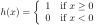
This algorithm is referred to in the literature as AdaBoost.M1 or Discrete AdaBoost (FHT00). The hypotheses $h_t(\mathbf{x})$ used by AdaBoost are features that can take only the values $\{+1,-1\}$.

The intuitive operation of AdaBoost is very simple: for each new classifier added to the sequence, AdaBoost focuses on the input patterns that have so far been classified least accurately.

AdaBoost has several interpretations: as a margin-maximizing classifier, as logistic regression applied to an additive model, as a discrete-step gradient-descent optimizer, and also as regression using Newton's method.

Like SVMs, AdaBoost maximizes the separation margin between classes, although using different metrics. Consequently, both methods are less sensitive to problems such as overfitting.