Multiclass Classification

The classifiers introduced so far have been presented primarily in the binary setting. In practice, however, many classification problems require distinguishing simultaneously between multiple categories. It is therefore necessary to extend the formalism of loss functions and linear classifiers to the multiclass case.

In the binary classification case considered in the previous sections, a linear classifier returns a single value

$$f(\mathbf{x}) = \mathbf{w}^{\top}\mathbf{x} + b$$ (5.63)

that determines on which side of the decision boundary the sample lies. In the multiclass case, with $K$ classes, it is instead necessary to associate a score with each class, yielding a vector

$$\mathbf{s} = f(\mathbf{x},\mathbf{W},\mathbf{b})$$ (5.64)

with

$$s_j = \mathbf{w}_j^{\top}\mathbf{x} + b_j, \qquad j=1,\ldots,K.$$ (5.65)

The scores $s_j$ do not necessarily represent probabilities, and their absolute values generally have no direct meaning. The classification problem therefore consists in comparing the scores of the different classes and assigning the sample to the class with the highest score.

In the multiclass case, it is likewise possible to define a loss function that quantifies how compatible the scores produced by the classifier are with the correct class. As discussed in Section 5.6, the choice of loss function substantially determines the criterion used to train the classifier.

One possibility is to extend to the multiclass case the concept of the hinge loss introduced for the SVM in Section 5.5. Let $y_i$ denote the correct class of the $i$-th sample and $s_j=f_j(\mathbf{x}_i)$ the score associated with class $j$. The multiclass SVM loss can then be defined as

$$\ell_i = \sum_{j \neq y_i} \max\left(0, s_j - s_{y_i} + 1\right).$$ (5.66)

The loss is zero when the score of the correct class exceeds that of every other class by at least a margin equal to $1$. Otherwise, every class that violates this margin is penalized. This formulation is therefore a natural extension of the binary hinge loss, in which the margin is evaluated with respect to all competing classes.

A variant is the squared hinge loss, in which the penalty is squared:

$$\ell_i = \sum_{j \neq y_i} \max\left(0, s_j - s_{y_i} + 1\right)^2.$$ (5.67)

The overall loss function can therefore be obtained as the mean of the losses over the samples, optionally with the addition of a regularization term:

$$\mathcal{L} = \frac{1}{n}\sum_{i=1}^{n}\ell_i + \lambda R(\mathbf{W}).$$ (5.68)

This formulation falls within the framework of empirical risk minimization introduced in Section 5.6. The term $R(\mathbf{W})$ makes it possible to penalize overly complex models and may, for example, correspond to L2 regularization of the weights.

Cross-entropy can naturally be extended to the multiclass case by introducing a probabilistic parameterization of the classes through the Softmax function.

The scores $s_j$ are transformed into probabilities through

$$p_j = \frac{e^{s_j}} {\sum_{k=1}^{K} e^{s_k}}.$$ (5.69)

The loss associated with the $i$-th sample is therefore the cross-entropy of the correct class:

$$\ell_i = -\log p_{y_i} = -\log \frac{e^{s_{y_i}}} {\sum_{j=1}^{K} e^{s_j}} = -s_{y_i} + \log\sum_{j=1}^{K}e^{s_j}.$$ (5.70)

This formulation is the multiclass extension of the cross-entropy introduced in Section 5.6. Since minimizing cross-entropy is equivalent to minimizing the negative log-likelihood of the observed class, the model can be interpreted as a maximum-likelihood estimator.

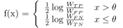
A regularization term can also be introduced in this case:

$$\mathcal{L} = -\frac{1}{n}\sum_{i=1}^{n} \log p_{y_i} + \lambda R(\mathbf{W}).$$ (5.71)

From a statistical point of view, the regularization term can be interpreted as introducing prior information about the model parameters. Under this interpretation, the estimate is no longer a simple maximum-likelihood estimate but a Maximum A Posteriori (MAP) estimate.

Loss functions therefore provide a common language for describing numerous classification algorithms. An alternative approach is to combine several simple classifiers to construct a more complex classifier, according to the Ensemble Learning paradigm.