Logistic Regression

Figure 4.2: Logistic Function

There is a family of linear models that relate the dependent variable to the explanatory variables through a nonlinear function, called generalized linear models (generalized linear model). Logistic regression belongs to this class of models in the particular case where the variable 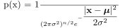$y$ is dichotomous, that is, can take only the values $0$ or $1$. By its nature, this type of problem is particularly important in classification problems.

For binary problems, it is possible to define the probabilities of success and failure:

$$\begin{array}{l} P[Y=1\vert\mathbf{x}]=p(\mathbf{x}) \\ P[Y=0\vert\mathbf{x}]=1-p(\mathbf{x}) \\ \end{array}$$ (4.113)

The response of a linear predictor of the form

$$y' = \boldsymbol\beta \cdot \mathbf{x} + \varepsilon$$ (4.114)

is not bounded between $0$ and $1$ and is therefore unsuitable for this purpose. It is necessary to associate the response of the linear predictor with the response of a certain function $g$, a function of the probability $p(\mathbf{x})$:

$$g(p(\mathbf{x}) ) = \boldsymbol\beta \cdot \mathbf{x} + b$$ (4.115)

where $g(p)$, the mean function, is a nonlinear function defined between $[0,1]$. $g(p)$ must be invertible, and its inverse $g^{-1}(y')$ is the link function.

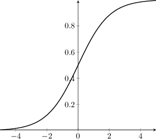
A widely used model for the function $g(p)$ is the logit function, defined as:

$$logit(p) = \log \frac{p}{1-p} = \boldsymbol\beta \cdot \mathbf{x}$$ (4.116)

The function $\frac{p}{1-p}$ represents how many times more likely success is than failure and is therefore called the odds ratio. Consequently, function (4.116) represents the logarithm of the probability that an event occurs relative to the probability that the same event does not occur (log-odds).

Its inverse exists and is given by

$$\E[Y\vert\mathbf{x}] = p( \mathbf{x} ) = \frac{ e^{\boldsymb... ...dot \mathbf{x}} }{ 1 + e^{\boldsymbol\beta \cdot \mathbf{x}} }$$ (4.117)

and is the logistic function.

In this case, the maximum-likelihood method does not coincide with the least-squares method, but with

$$\mathcal{L}(\boldsymbol\beta) = \prod_{i=1}^{n} f(y_i\vert \... ...y_i} ( \mathbf{x}_i) \left(1 - p^{y_i} ( \mathbf{x}_i) \right)$$ (4.118)

which gives the log-likelihood function

$$\log \mathcal{L}(\boldsymbol\beta) = \sum_{i=1}^{n} y_i (\bo... ...log \left( 1 + e^{\boldsymbol\beta \cdot \mathbf{x}_i} \right)$$ (4.119)

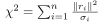whose maximization through iterative techniques allows the parameters $\boldsymbol\beta$ to be estimated.