Particle Filter

The linear and quasi-linear approaches proposed by Kalman can be used for problems in which the state is Gaussian or approximately Gaussian with a unimodal distribution: the state estimate at time $k$ is a direct function of the single state estimate at time $k-1$ and of the covariance of that estimate.

When it is necessary to obtain the non-Gaussian probability distribution of the system state $p(x_k; u_{k-1}; z_{k})$ at time $k$ as a function of the inputs and observations, Kalman-type approaches are no longer adequate.

Grid-based approaches are suitable for problems, which are uncommon in practice, in which the state is finite and discretizable. Histogram Filters/Occupancy Grid Methods apply to a broader class of problems, but because of the uniform sampling of the state, they scale very poorly as the dimensionality increases.

Consider again the result expressed by equation (2.4): to extract a generic statistic $h(\cdot)$ (for example, the mean or variance) from a probability distribution $p(x)$, the expression

$$\bar{h} \stackrel{def}{=} \int_X h(x) p(x) dx$$ (3.41)

is used. When this estimate cannot be obtained analytically, it can nevertheless be computed indirectly by analyzing $x_i$ independent samples, with $1 \leq i \leq N$, drawn randomly from the exact distribution $p$.

Given the samples $x_i$ generated in this way, the Monte Carlo estimate of $h(\cdot)$ is

$$\bar{h} \approx \frac{1}{N} \sum_{i=1}^{N} h(x_i)$$ (3.42)

Monte Carlo methods do not solve every problem, nor do they indicate how to obtain random samples efficiently. The problem becomes significant in multidimensional cases, where the regions in which the probability takes significant values are extremely small. The objective of Importance Sampling (IS) is precisely to sample the distribution $p(x)$ in “important” regions in order to maximize computational efficiency.

The idea behind Importance Sampling is to use a simpler distribution 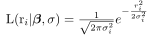$q(x)$ (importance density) in place of the true distribution $p(x)$, which is normally difficult to sample from (or reproduce), making the substitution

$$\int_X h(x) p(x) dx = \int_X h(x) \frac{p(x)}{q(x)} q(x) dx = \int_X h(x) w(x) q(x) dx$$

and introducing the system of weights $w(x)$.

By using suitable weights, equation (3.42) can therefore be rewritten as

$$\bar{h} \approx \sum_{i=1}^{N} w_i h(x_i)$$ (3.43)

where

$$W_i = \frac{p(x_i)}{q(x_i)}$$

represents a correction factor, called the importance weight, for converting the proposal distribution $q$ into the true distribution $p$. The weights are then normalized

$$w_i = \frac{W_i} {\sum_{j=1}^{N} W_j}$$ (3.44)

so that

$$\sum_{i=1}^{N} w_i = 1.$$

The closer the distribution $q(x)$ is to $p(x)$ in the regions of highest probability, the lower the variance of the weights and the more efficient the estimate. On the other hand, the distribution $q(x)$ must be very easy to sample from, for example by choosing a uniform or Gaussian distribution.

Given knowledge of Bayesian filters and Monte Carlo techniques, it is possible to develop the theory of particle filters. The state at time $k$ is represented by a set of samples (particles), and each sample is a hypothesis of the state to be evaluated. One can consider a set of particles obtained a priori to the observation by applying equation (3.43) to the state-evolution function.

By applying Bayesian theory directly to samples from the estimated distribution, it is possible to modify the weights $w_i$ associated with the samples using both the system and perception models (Sequential Importance Sampling):

$$w_{k,i} \propto w_{k-1,i} \frac{ p (z_k \vert x_{k,i} ) p (x_{k,i} \vert x_{k-1,i} ) } { q (x_{k,i} \vert x_{k-1,i}, z_k ) }$$ (3.45)

At each iteration, the particles are propagated according to the proposal distribution $q(\cdot)$, and their weights $w_i$ are updated recursively according to equation (3.45).

When possible, it is convenient to use the a priori distribution as the importance density

$$q (x_{k,i} \vert x_{k-1,i}, z_k ) = p (x_{k,i} \vert x_{k-1,i} )$$ (3.46)

so that, when substituted into (3.45), it gives

$$w_{k,i} \propto w_{k-1,i} p (z_k \vert x_{k,i} )$$ (3.47)

The problem with the SIS approach is that, after a few iterations, only a few particles have a non-negligible weight factor (weight degeneracy).