M-Estimator

The use of least-squares regression (Least squares) for the error, rather than other weighting functions, is motivated both by the maximum-likelihood function and, above all, by the simplicity of the derivatives obtained in the Jacobian.

In the problems considered so far, the variance has almost always been assumed to be constant, with observation errors distributed according to a normal distribution. If the noise were purely Gaussian, this approach would be theoretically correct; however, real applications usually involve distributions consisting of Gaussian noise associated with the model and noise associated with elements that do not belong to the model itself (outliers). Under these conditions, least-squares regression treats all points as if the error were Gaussian, assigning little weight to points close to the model and much greater weight to points far from the model, which, purely on probabilistic grounds, are usually outliers.

A unified way of handling these problems was introduced by John Nelder, who named these techniques generalized linear models (GLM, General Linear Models).

To solve this problem, the metric used to evaluate the errors must be changed: a first example of a different metric that could solve the problem is least-absolute-value regression. However, minimizing an error function expressed as an absolute-value distance (Least absolute deviations regression) is not easy, because its derivative is discontinuous and requires iterative optimization techniques; differentiable metrics are preferable in this case.

In 1964, Peter Huber proposed a generalization of the concept of maximum-likelihood minimization by introducing M-estimators.

Some examples of regression functions are shown in Figure 4.3.

Figure 4.3: Examples of weighting functions for regression: least-squares regression (L2 metric), linear regression (L1), Huber estimators, Tukey's biweight, the Lorentzian (Cauchy) function, and the Welsch (Leclerc) function.

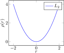
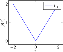
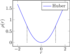
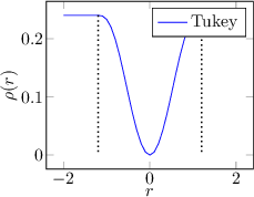
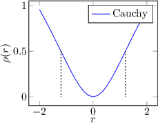
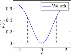
An M-estimator replaces the sum-of-squares metric with a metric based on a generic $\rho$ function (loss function) having a unique minimum at zero and subquadratic growth. M-estimators generalize least-squares regression: setting $\rho(\mathbf{r})=\Vert\mathbf{r}\Vert^2$ yields the classical form of regression.

Finally, if the loss function is monotonically increasing, the estimator is called an M-estimator; if the loss function increases near zero but decreases far from zero, it is called a redescending M-estimator.

The parameters are estimated by minimizing a sum of generic weighted quantities:

$$\min_\beta \sum \rho \left( \frac{\mathbf{r}_i}{\sigma_i} \right)$$ (4.125)

whose closed-form or iterative solution differs from the least-squares solution because of the different derivative of the function $\rho$:

$$\sum_{i=1}^{n} \frac{1}{\sigma_i} \rho' \left( \frac{\mathbf... ...artial \mathbf{r}_i}{\partial \beta_j} = 0 \qquad j=1,\ldots,m$$ (4.126)