Levenberg-Marquardt

In the preceding sections, algorithms for solving nonlinear systems were divided into gradient-descent methods and Gauss-Newton methods. For a more detailed treatment, see (MBT04).

In Gauss-Newton methods, when $\mathbf{J}^{\top}\mathbf{J}$ is positive definite, the method always provides a descent direction for the cost function. However, when $\mathbf{J}^{\top}\mathbf{J}$ becomes singular, the method may become numerically unstable.

The technique proposed by Levenberg-Marquardt attempts to combine the strengths of Gauss-Newton and gradient descent, taking advantage of both.

The Levenberg-Marquardt (LM) algorithm is an iterative technique now considered standard for solving multivariate nonlinear problems. A detailed description of the algorithm is available in (Lou05).

LM can be viewed as consisting of an initial gradient-descent phase, which is slower but stable, followed by a Gauss-Newton-type solver, which is faster but less robust.

The algorithm solves a modified version of equation (4.49), a special case of equation (4.35), known as the augmented normal equations:

$$\mathbf{N} \boldsymbol\delta_\beta = -\mathbf{J}_{r}^{\top} \mathbf{r}$$ (4.53)

where $\mathbf{N} = \mathbf{H}_{S} + \mu \mathbf{I}$ and $\mu > 0$ is a damping factor. When $\mu$ is large, $\mathbf{N}$ is nearly diagonal and the algorithm behaves like gradient descent. When $\mu$ is close to zero, LM approximates Newton's method.

Unlike line search, LM implements the concept of a trust region, dynamically adapting the region within which the model linearization is assumed to be valid.

As in the Gauss-Newton method, LM exploits the Hessian approximation:

$$\mathbf{H}_S(\boldsymbol\beta) \approx \mathbf{J}_{r}^{\top}\mathbf{J}_{r}$$ (4.54)

which is valid when the loss function is quadratic.

The initial choice and the update of parameter $\mu$ between iterations are left to the solver, and several strategies have been proposed in the literature.

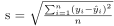
One of the most widely used implementations (Nie99) initializes $\mu$ as:

$$\mu_0 = \tau \max \trace \mathbf{H}$$ (4.55)

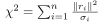
where $\tau$ is freely chosen by the user based on the confidence in the initial estimate of $\boldsymbol\beta$.

The update of $\mu$ is guided by the gain ratio $\rho$:

$$\rho = \frac{ S(\boldsymbol\beta) - S(\boldsymbol\beta + \bo... ...\mu \boldsymbol\delta_\beta + \mathbf{J}^{\top} \mathbf{r} ) }$$ (4.56)

A high value of $\rho$ indicates that the model linearization is effective, and $\mu$ can be reduced. Conversely, if $\rho$ is low or negative, $\mu$ must be increased to approach gradient-descent behavior. When $\rho \approx 1$, there is good agreement between the model and the data.

The update of $\mu$ can be managed according to the following rule: