


Next: Linear Least-Squares Regression Up: Regression and Optimization Methods Previous: The Cramer-Rao Bound
We first examine the most common case in real-world applications, in which the observation noise is additive white Gaussian noise.
Let
 and some inputs
  , to which additive zero-mean Gaussian noise with variance
  is added.
To estimate the parameters robustly, the number of input samples
is added.
To estimate the parameters robustly, the number of input samples
 must be large, much larger than the number of parameters.
The parameter function need not be the same for all samples; different functions may instead be used, effectively measuring different quantities that are all functions of the same parameters
.
In this case, equation (4.2) can be generalized as
 implicitly denotes both the type of function and the -th input sample (in fact, a constant parameter of the function).
The vector 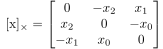 is introduced, defined as
 |
(4.4) |
-th observation (or with the -th function).
 is a function of
, just as
is a function of
, just as  is, and shares its derivatives with it (apart from a sign under this notation).
To obtain a maximum-likelihood estimator, the quantity to minimize is the negative log likelihood (Section 2.7) of function (4.2).
For Gaussian noise, the likelihood function is in fact written as
Least-squares regression is a standard optimization technique for overdetermined systems that identifies the parameters
 of a function
 minimizing an error
  computed as the sum of the squares (Sum Of Squared Error) of the residuals over a set of
 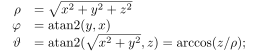 observations
 :
:
 is defined as the residual sum of squares or, alternatively, as the expected squared error.
 is a function analyzed as the parameters
 vary in order to find its minimum value
From a purely computational standpoint, finding a global minimum is difficult, and techniques that identify only local minima are normally used.
Let
4.1 be differentiable, that is, let  be differentiable.
A necessary condition for
to be a minimum is that, at that point in parameter space, the gradient of
vanish, namely
be differentiable.
A necessary condition for
to be a minimum is that, at that point in parameter space, the gradient of
vanish, namely
A sufficient condition for a stationary point (
 ) to be a minimum is that
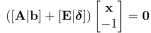 (the Hessian) be positive definite.
Clearly, the existence of a local minimum only guarantees that there exists a neighborhood
(the Hessian) be positive definite.
Clearly, the existence of a local minimum only guarantees that there exists a neighborhood  of
such that the function
of
such that the function
 .
.
The discussion so far has assumed that the noise is additive  with constant variance across all samples (homoscedasticity).
When the measurement noise is still zero-mean additive Gaussian noise but has nonconstant variance, each observation
with constant variance across all samples (homoscedasticity).
When the measurement noise is still zero-mean additive Gaussian noise but has nonconstant variance, each observation  is an independent random variable associated with variance
  .
It is intuitive that, in this case, the optimal regression should assign greater weight to samples with low variance and lower weight to samples with high variance.
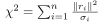
To obtain this result, a normalization is used, similar to that shown in Section 2.4.1 and resulting directly from the likelihood in equation (4.5). Therefore, the simple sum of squared residuals must no longer be minimized; instead, the weighted sum of residuals must be minimized:
.
It is intuitive that, in this case, the optimal regression should assign greater weight to samples with low variance and lower weight to samples with high variance.
To obtain this result, a normalization is used, similar to that shown in Section 2.4.1 and resulting directly from the likelihood in equation (4.5). Therefore, the simple sum of squared residuals must no longer be minimized; instead, the weighted sum of residuals must be minimized:
 |
(4.9) |
 .
The minimum of this cost function coincides with that previously obtained by least squares when the variance is constant.
Condition (4.8) for obtaining the minimum is modified accordingly:
.
The minimum of this cost function coincides with that previously obtained by least squares when the variance is constant.
Condition (4.8) for obtaining the minimum is modified accordingly:
Generalizing this concept further, when the observation is affected by Gaussian noise with known covariance matrix
 , the Weighted Sum of Squared Error (WSSE) can finally be written as
 |
(4.11) |
Any Weighted Least Squares problem can be reduced to an unweighted problem
 by premultiplying the residuals (and consequently the derivatives) by a matrix
 such that
 , using, for example, a Cholesky decomposition when this matrix is not diagonal.
All these estimators, which account for the variance of the observation, coincide with the negative log likelihood for the variable  perturbed by zero-mean Gaussian noise with covariance
.
perturbed by zero-mean Gaussian noise with covariance
.
is often defined with a scaling factor  so that the gradient of is not affected by the factor
  and has the same sign as , thereby simplifying the notation.



