State Estimation and Bayesian Filters

This chapter discusses the problem of statistical filtering, namely, the class of problems in which data from one or more noisy sensors are available. These data represent observations of the dynamic state of a system that is not directly observable but whose state must be estimated. The procedure used to find the best estimate of a system's internal state is called “filtering” because it filters out the various noise components. The evolution of a system (that is, the evolution of its internal state) must follow known physical laws, which are affected by a noise component (process noise). Knowledge of the equations governing state evolution makes it possible to obtain a better estimate of the internal state.

A physical process can be represented in state space (State Space Model) by a function describing how the state $\mathbf{x}_t$ evolves over time:

$$\dot{\mathbf{x}}_t = f(t, \mathbf{x}_t, \mathbf{u}_t, \mathbf{w}_t)$$ (3.1)

where $\mathbf{u}_t$ denotes any known inputs to the system, and $\mathbf{w}_t$ is a parameter representing process noise, that is, the randomness governing the evolution of the system. Similarly, state observation is also a process affected by noise, in this case referred to as observation noise. Here too, it is possible to define a function modeling the observation $\mathbf{z}_t$ as

$$\mathbf{z}_t = h (t, \mathbf{x}_t, \mathbf{v}_t )$$ (3.2)

where $\mathbf{v}_t$ is observation noise and the function depends only on the current state.

This formalism is described in the continuous-time domain. In practical applications, signals are sampled at discrete times $k$, and a discrete-time version is therefore normally used, in the form

$$\begin{array}{l} x_{k+1} = f_k(x_k, u_k, w_k) \\ z_{k+1} = h_k(x_k, v_k) \\ \end{array}$$ (3.3)

where $w_k$ and $v_k$ can be regarded as white-noise sequences with known statistics.

Figure 3.1: Example of the evolution and observation of a Markovian system.

In systems satisfying equations (3.3), state evolution depends only on the previous state, whereas observation depends only on the current state (Figure 3.1). If a system satisfies these assumptions, the process is said to be Markovian: system evolution and observation depend only on the current state, not on past states. Access to state information is always indirect, through observation (Hidden Markov Model).

Many approaches for estimating the unknown state of a system from a set of measurements do not account for the noisy nature of these observations. It is possible, for example, to construct an algorithm that performs nonlinear regression on the observations to estimate all the states in the problem by solving an optimization problem with a large number of unknowns.

Unlike regression methods, filters aim to provide the best estimate of the variables (state) as observation data become available. From a theoretical standpoint, regression provides the optimal result, whereas filtering converges to the correct result only after a sufficiently large number of samples.

Bayesian filters aim to estimate, at discrete time $k$, the state of the random variable $\mathbf{x}_k \in \mathbb{R}^n$ given an indirect observation of the system, $\mathbf{z}_k \in \mathbb{R}^{m}$.

Filtering techniques make it possible both to obtain the best estimate of the unknown state 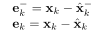$\mathbf{x}_k$ and to determine the multivariate probability distribution 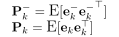$p(\mathbf{x}_k)$ representing the available knowledge of that state.

Given an observation of the system, it is possible to define the probability density of $\mathbf{x}_k$ a posteriori with respect to observation of the event $\mathbf{z}_{k}$, based on the additional information provided by that observation:

$$p^{+}(\mathbf{x}_k) = p(\mathbf{x}_k \vert \mathbf{z}_k)$$ (3.4)

where the conditional probability $p(\mathbf{x}_k \vert \mathbf{z}_k)$ denotes the probability that the hidden state is $\mathbf{x}_k$ given the observation $\mathbf{z}_k$. The “function” $p(\mathbf{x}_k \vert \mathbf{z}_k)$ represents the state measurement model (measurement model). In the literature, the posterior distribution $p^{+}(\mathbf{x}_k)$ is also referred to as the belief.

Applying Bayes' theorem to equation (3.4) gives

$$p(\mathbf{x}_k \vert \mathbf{z}_k) = c_k p(\mathbf{z}_k \vert \mathbf{x}_k) p(\mathbf{x}_{k})$$ (3.5)

where $c_k$ is a normalization factor such that $\int p(\mathbf{x}_k \vert \mathbf{z}_k)=1$. Knowledge of $p(\mathbf{z}_k \vert \mathbf{x}_k)$ is essential: it represents the probability that the observation is precisely the quantity $\mathbf{z}_k$ observed given the possible state $\mathbf{x}_k$. The use of Bayes' theorem to estimate the state given an observation is why this class of filters is called Bayesian.

In addition to posterior knowledge of the probability distribution, further information can be used to improve the estimate: prior knowledge with respect to the observation, obtained from the constraint that the state does not evolve in a completely unpredictable manner but can instead evolve only in certain ways with certain probabilities. These possible modes of system evolution depend only on the current state. The Markov assumption implies that the only past state affecting system evolution is the state at time $k-1$, namely $p(x_k \vert x_{1:k-1}) = p(x_k \vert x_{k-1})$.

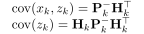
It is therefore possible to perform an a priori prediction using the Chapman–Kolmogorov equation:

$$p^{-}(\mathbf{x}_k) = \int p(\mathbf{x}_k \vert \mathbf{x}_{k-1}, \mathbf{u}_{k}) p(\mathbf{x}_{k-1}) d\mathbf{x}_{k-1}$$ (3.6)

where $p(\mathbf{x}_k \vert \mathbf{x}_{k-1}, \mathbf{u}_{k})$ represents the system dynamics (dynamic model) and $\mathbf{u}_{k}$ denotes any inputs that influence system evolution and are assumed to be completely known.

Given the prior state estimate and the observation 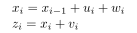$z_k$, equation (3.4) can be rewritten as the state-update equation

$$p^{+}(\mathbf{x}_k) = c_k p(\mathbf{z}_k \vert \mathbf{x}_k) p^{-}(\mathbf{x}_k)$$ (3.7)

The state is estimated by alternating a prediction phase (prior estimate) with an observation phase (posterior estimate). This iterative process is called recursive Bayesian estimation (Recursive Bayesian Estimation).

The techniques described in this section use only the latest available observation to estimate the state. Formally, the discussion can be extended to the case in which all observations are used to obtain a more accurate state estimate. In this case, the filtering and prediction equations become

$$\begin{array}{l} p(\mathbf{x}_k \vert \mathbf{z}_{1:k} ) = ... ...mathbf{x}_k \vert \mathbf{z}_{1:k} ) d \mathbf{x}_k \end{array}$$ (3.8)

For simplicity and because of the lower computational cost, only the latest observation is normally considered. In certain cases, however, such as particle filters, knowledge of the entire history can be incorporated into the equations relatively easily.

Since the variables to be estimated are continuous, Bayesian theory cannot be used “directly.” Several approaches have therefore been proposed in the literature to enable efficient estimation, both computationally and in terms of memory usage.

Depending on whether the problem is linear or nonlinear and whether the noise probability distribution is Gaussian, each of these filters performs with varying degrees of optimality.

The Kalman filter (Section 3.2) is optimal when the problem is linear and the noise distribution is Gaussian. The Extended Kalman and Sigma-Point filters, Sections 3.4 and 3.5, respectively, are suboptimal filters for nonlinear problems with Gaussian noise distributions, or distributions that deviate only slightly from Gaussian. Finally, particle filters are a suboptimal solution for nonlinear problems with non-Gaussian noise distributions.

Grid-based filters (Section 3.1) and particle filters (Section 3.8) operate on a discrete representation of the state, whereas Kalman, Extended Kalman, and Sigma-Point filters operate on a continuous representation.

Kalman, Extended Kalman, and Sigma-Point filters estimate the uncertainty distribution (of the state, process, or observation) as a single Gaussian. Multimodal extensions such as Multi-hypothesis tracking (MHT) make it possible to apply Kalman filters to distributions such as Gaussian mixtures, whereas particle and grid-based filters are inherently multimodal.

An excellent survey of Bayesian filtering is (Che03).