Normal equations

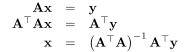
A first way to obtain the least-squares solution is to differentiate the error function with respect to $\mathbf {x}$:

$$\frac{\partial \epsilon}{\partial\mathbf{x}} = 2\mathbf{A}^{\top} \left(\mathbf{A}\mathbf{x}-\mathbf{y}\right).$$ (1.4)

Setting this derivative equal to zero gives

$$\mathbf{A}^{\top}\mathbf{A}\mathbf{x} = \mathbf{A}^{\top}\mathbf{y}.$$ (1.5)

These are referred to in the literature as the normal equations: the original problem is reduced to a square linear system.

If $\mathbf{A}$ has full column rank, that is, $\operatorname{rank}(\mathbf{A})=n$, the matrix $\mathbf{A}^{\top}\mathbf{A}$ is positive definite and invertible. In this case, the solution is

$$\hat{\mathbf{x}} = \left(\mathbf{A}^{\top}\mathbf{A}\right)^{-1} \mathbf{A}^{\top}\mathbf{y}.$$ (1.6)

The matrix $\mathbf{A}^{\top}\mathbf{A}$ is symmetric and, in the case of full column rank, positive definite; the normal equations can therefore be solved using a Cholesky factorization. However, explicitly forming $\mathbf{A}^{\top}\mathbf{A}$ has a numerical disadvantage: in the 2-norm, the condition number satisfies

$$\kappa_2\left(\mathbf{A}^{\top}\mathbf{A}\right) = \kappa_2(\mathbf{A})^2.$$ (1.7)

The conditioning of the problem is therefore worsened by forming the normal equations. Further details on matrix conditioning and the propagation of perturbations in the solution of linear systems are presented in section 1.2.