Determination of the Matrices

The Essential Matrix can be obtained in closed form when the relative poses between the sensors are known; with knowledge of the intrinsic parameters of the cameras involved, the Fundamental Matrix can then be obtained.

The most widespread application of the Essential (or Fundamental) Matrix, however, is to recover the relative pose between the cameras from a set of corresponding points: when the intrinsic parameters are known, the Essential Matrix can be recovered (and the Fundamental Matrix can then be obtained from it); without any knowledge of the camera parameters, the Fundamental Matrix can be recovered directly.

The 8-Point Algorithm

The criterion for obtaining matrix $\mathbf{F}$ can be formalized as the minimization of a cost function

$$\min_\mathbf{F} \sum_{i=1}^n \left( \mathbf{p}^{\top}_{2,i} \mathbf{ F } \mathbf{p}_{1,i} \right)^2$$ (10.51)

subject to additional constraints, this time concerning the structure of $\mathbf{F}$.

It can be noted that the epipolar constraint (10.47) can also be rewritten as

$$(\mathbf{p}_1 \otimes \mathbf{p}_2)^{\top} \text{vec}(\mathbf{F}) = 0$$ (10.52)

by exploiting the compact notation provided by the Kronecker product $\otimes$, or alternatively

$$\mathbf{u}_i \mathbf{f} = 0$$ (10.53)

in a more explicit form by defining

$$\begin{array}{rl} \left( \mathbf{p}_1 \otimes \mathbf{p}_2 \... ...,3} , f_{3,1} , f_{3,2} , f_{3,3} \right)^{\top} \end{array}$$ (10.54)

with $\mathbf{p}_{1,i}=(x_1,y_1)$ and $\mathbf{p}_{2,i}=(x_2,y_2)$. With this formalism, it is possible to highlight a technique for obtaining the elements of $\mathbf{F}$ as the solution of a homogeneous linear system formed by constraints such as the one in equation (10.53).

Collecting all the constraints 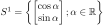$\mathbf{u}_i$ yields a homogeneous system of the form

$$\mathbf{U} \mathbf{f} = 0$$ (10.55)

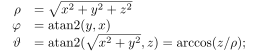with $n$ equations in 9 unknowns.

The derivation for obtaining the Essential Matrix is analogous: it is the solution of a system $\mathbf{n}_i \mathbf{e}=0$ of the form

$$\begin{array}{l} \mathbf{n}_i = ( x_{1} x_{2}, y_{1} x_{2... ..._{2,2} , e_{2,3} , e_{3,1} , e_{3,2} , e_{3,3} ) \end{array}$$ (10.56)

with $\mathbf{m}_{1,i}=(x_1,y_1,z_1)$ and $\mathbf{m}_{2,i}=(x_2,y_2,z_2)$. With all the constraints $\mathbf{n}_i$, this is a homogeneous system of the form

$$\mathbf{N} \mathbf{e} = 0$$ (10.57)

In fact, when homogeneous coordinates are used, systems (10.54) and (10.56) are algorithmically equivalent.

One additional constraint must always be added to the constraints expressed in these homogeneous systems, for example $\Vert \mathbf{f} \Vert =1$, which is normally already satisfied by linear solvers for homogeneous systems. This algorithm is therefore called the eight-point algorithm, since at least 8 points are required to determine the solution. Additional constraints needed to reach the actual degrees of freedom of the matrices, however, cannot be expressed in linear form.

Constraint Enforcement

Because of noise, the matrices obtained from the linear system normally do not satisfy the requirement that they have rank 2; in the case of the Essential Matrix, which has a larger number of degrees of freedom, they may not even belong to the subspace of Essential Matrices. One possible solution is to seek the matrix closest to the one returned by the linear system that nevertheless satisfies the rank constraint. This result can be obtained, for example, by using an SVD followed by a composition, as suggested by Tsai, Huang, and Hartley:

$$\begin{array}{rl} \mathbf{F} &= \mathbf{U}\diag (r,s,t)\ma... ...bf{F}' &= \mathbf{U}\diag (r,s,0)\mathbf{V}^{\top} \end{array}$$ (10.58)

This procedure is called constraint enforcement. Compared with the Fundamental Matrix, the Essential Matrix has the additional constraint that its 2 nonzero singular values be equal:

$$\begin{array}{rl} \mathbf{E} &= \mathbf{U}\diag (r,s,t)\ma... ...bf{E}' &= \mathbf{U}\diag (1,1,0)\mathbf{V}^{\top} \end{array}$$ (10.59)

If the singular values of the matrix, following an SVD, are 1, the matrix is called a normalized Essential Matrix (normalized essential matrix). The Essential Matrix obtained by setting $\mathbf{D}' = \diag (1, 1, 0)$ is the normalized Essential Matrix closest to the given one according to the Frobenius norm. The Essential Matrix generated through equation (10.59) satisfies the cubic trace-constraint (Demazure, 1988):

$$\mathbf{E}\mathbf{E}^{\top} \mathbf{E} - \frac{1}{2} \trace \left( \mathbf{E}\mathbf{E}^{\top} \right) \mathbf{E} = 0$$ (10.60)

This constraint is a necessary condition for the matrix under consideration to be an Essential Matrix.

The matrices obtained through this enforcement procedure satisfy all the requirements for being Fundamental or Essential Matrices, but they do not represent an algebraic, let alone geometric, minimization of the original constraints.

The 7-Point Algorithm

Algorithms that use fewer than 8 points to extract an Essential or Fundamental Matrix are based more or less on the same principle: the multidimensional kernel of $\mathbf{U}$ or $\mathbf{N}$ is extracted, since the Fundamental or Essential Matrix must belong to an element of this space, and some constraints specific to the problem are enforced.

In the nonlinear case, it is relatively easy to obtain a Fundamental Matrix from only 7 points, given that matrix $\mathbf{U}$, formed from the elements in equation (10.54), must have rank 7, since the Fundamental Matrix has exactly 7 degrees of freedom. Solving system (10.54) formed from (at least) 7 points yields a two-dimensional subspace, formed by two bases $\mathbf{f}_1$ and $\mathbf{f}_2$, associated with two matrices $\mathbf{F}_1$ and $\mathbf{F}_2$. Within the space of possible solutions, it is necessary to find a matrix $\mathbf{F} = \alpha \mathbf{F}_1 + (1 - \alpha) \mathbf{F}_2$ having rank 2, that is, by imposing $\det \mathbf{F} = 0$, a third-degree nonlinear equation in $\alpha$. In this case, the real solutions of $\alpha$ may number 1 or 3. If there are 3 real solutions, all three must be evaluated on the data to identify the most plausible one.

The 5-Point Algorithm

With fewer than 7 points, only algorithms for determining the Essential Matrix exist. The Essential Matrix has only 5 degrees of freedom and can, in theory, be estimated by analyzing correspondences between just 5 points (Nis04). The 5-point algorithm is in fact the standard method for estimating the Essential Matrix; however, its implementation is extremely complex.

Using only 5 correspondences, matrix $\mathbf{N}$ of system (10.57) has a rank deficiency of 4. The Essential Matrix must therefore be expressed as a linear combination of the last 4 columns of matrix $V$ obtained from the SVD, namely:

$$\mathbf{E} = x \mathbf{X} + y \mathbf{Y} + z \mathbf{Z} + \mathbf{W}$$ (10.61)

where $\left(\mathbf{X}, \mathbf{Y}, \mathbf{Z}, \mathbf{W}\right)$ are the last 4 columns of eigenvectors of matrix $V$ and $(x,y,z)$ are unknowns. To obtain these unknowns, it is necessary to satisfy the constraints

$$\begin{array}{l} \det \mathbf{E} = 0 \\ \mathbf{E}\mathbf... ...thbf{E}\mathbf{E}^{\top} \right) \mathbf{E} = 0 \\ \end{array}$$ (10.62)

which is equivalent to a problem involving 10 third-degree polynomials in the 3 unknowns.

The need to solve a nonlinear system nevertheless reduces the advantages over the solutions proposed in Section 10.4.2.

System Conditioning

The generation of the Essential and Fundamental Matrices using SVD, followed by their enforcement through equalization of the singular values, is highly sensitive to noise.

Matrix (10.54) is ill-conditioned. This occurs when one attempts to solve a linear system whose right-hand-side terms contain numbers with different orders of magnitude. The method proposed by Hartley (Har95) improves the solution by normalizing the point coordinates.

Coordinates $\mathbf {p}_1$ and $\mathbf {p}_2$ are translated separately so that their centroids are at the origin, and rescaled so that their mean value is $1$ (or $\sqrt{2}$, the mean modulus) in the new coordinate systems $\tilde{\mathbf{p}}_1$ and $\tilde{\mathbf{p}}_2$, respectively. We therefore define two transformation matrices $\mathbf{T}_1$ and $\mathbf{T}_2$ such that

$$\begin{array}{l} \tilde{\mathbf{p}}_1 = \mathbf{T}_1 \math... ...ilde{\mathbf{p}}_2 = \mathbf{T}_2 \mathbf{p}_2 \\ \end{array}$$ (10.63)

In this way, it is possible to determine the compatible Fundamental Matrix $\tilde{\mathbf{F}}$:

$$\mathbf{p}^{\top}_{2} \mathbf{ F } \mathbf{p}_1 = \tilde{\m... ...thbf{p}}_2^{\top} \tilde{\mathbf{F}} \tilde{\mathbf{p}}_1 = 0$$ (10.64)

from which the original matrix $\mathbf{F} = \mathbf{T}^{\top}_2 \tilde{\mathbf{F}} \mathbf{T}_1$ can then be recovered.