MLE computation of the homography

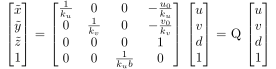
From a computational standpoint, Equation (9.57) is ill-conditioned because each column represents a quantity with a different order of magnitude. A prior normalization step is required to obtain a correct solution from the linear formulation. Hartley and Zisserman (HZ04) emphasize that normalization in DLT is an essential step and cannot be regarded as merely optional.

However, computing the homography in Equation (9.58) has the drawback that it does not account for measurement error in the points. In fact, SVD minimizes a quantity that, purely by chance, resembles the error in the known term (which is not what is minimized in case (9.57)), and in any event it is not possible to evaluate the error in the parameter matrix. In this specific case, where a purely mathematical error with no corresponding geometric interpretation is minimized in the least-squares sense, the method is called algebraic least squares (ALS).

Since DLT minimizes an algebraic rather than a geometric error, normalized DLT may produce worse results in terms of geometric data fitting, even though it is computationally superior. The normalized least-squares version of system (9.57) is called normalized algebraic least squares (NALS).

To overcome the limitation of algebraic-error minimization, it is necessary to return to the original problem rather than transform it into a linear one, and instead solve it, for example iteratively, using a nonlinear minimizer.

If noise is present in only one of the two images, an appropriate cost function with a geometric meaning is the Euclidean distance between the measured points and the transformed points. This is normally called the transfer error and minimizes a nonlinear cost function of the form

$$\argmin_\mathbf{H} \sum \Vert \mathbf{m}'_i - \mathbf{H} \mathbf{m}_i \Vert^2$$ (9.63)

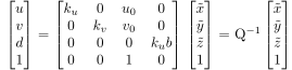where $\mathbf{m}'_i$ is the image point affected by white Gaussian noise, while point $\mathbf{m}_i$ is known exactly. In this case, the function that minimizes the geometric error is also the one that provides the best estimate from a Bayesian perspective (Maximum Likelihood Estimator, or MLE).

However, when both data sets are affected by noise, cost function (9.63) is not optimal. The simplest way to extend the previous solution is to minimize both the direct transfer error and the inverse transfer error (symmetric transfer error):

$$\argmin_\mathbf{H} \sum \Vert \mathbf{m}'_i - \mathbf{H} \m... ... + \Vert \mathbf{m}_i - \mathbf{H}^{-1} \mathbf{m}'_i \Vert^2$$ (9.64)

In this way, both contributions are taken into account when solving the problem.

This is not yet the optimal solution, at least from a statistical standpoint. A maximum-likelihood estimator must correctly account for the noise in both data sets when present (what Hartley and Zisserman call the Gold Standard). The alternative solution, and in fact the more accurate one, consists in minimizing the reprojection error.

This solution greatly increases the dimensionality of the problem because it also aims to identify, or includes among the unknowns, the optimal noise-free points $\hat{\mathbf{m}}_i$ and $\hat{\mathbf{m}}'_i$:

$$\argmin_\mathbf{H} \sum \Vert \mathbf{m}'_i - \hat{\mathbf{m}}'_i \Vert^2 + \Vert \mathbf{m}_i - \hat{\mathbf{m}}_i \Vert^2$$ (9.65)

subject to constraint $\hat{\mathbf{m}'}_i = \mathbf{H} \hat{\mathbf{m}}_i$.

In the even more general case in which the noise covariance is measured for each individual point, the correct metric is the Mahalanobis distance (see Section 2.4):

$$\Vert \mathbf{m} - \hat{\mathbf{m}} \Vert^{2}_{\Gamma} = (\... ...athbf{m}})^{\top} \Gamma^{-1} (\mathbf{m} - \hat{\mathbf{m}})$$ (9.66)

When the noise is constant for each point, the preceding expression reduces to the more intuitive Euclidean distance.

Since this is a nonlinear minimization, an initial solution is nevertheless required from which to search for the minimum satisfying the cost equation. The linear solution remains useful and is used as the initial estimate for finding a minimum under a different metric.

The MLE estimator requires one additional auxiliary variable $\hat{\mathbf{m}}_i$ for each point, as well as iterative techniques to solve the problem. The Sampson error can be used as an approximation of the geometric distance; see Section 4.3.8. The homographic constraint (1.111) relating the points in the two images can be written in the form of a two-dimensional $\mathcal{V}_H$ variety:

$$\begin{array}{l} h_0 u_1 + h_1 v_1 + h_2 - h_6 u_1 u_2 - h_... ...+ h_5 - h_6 u_1 v_2 - h_7 v_1 v_2 - h_8 v_2 = 0 \\ \end{array}$$ (9.67)

and therefore the Jacobian is

$$\mathbf{J}_\mathcal{V} = \begin{bmatrix} h_0 - h_6 u_2 & h_... ...& h_4 - h_7 v_2 & 0 & -h_6 u_1 -h_7 v_1 - h_8 \\ \end{bmatrix}$$ (9.68)

to be used when computing the Sampson distance (CPS05).

Error propagation in homography computation

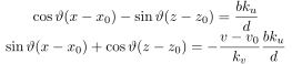
In the case of error in a single image, to determine how the error propagates to matrix $\mathbf{H}$, it is necessary to calculate the Jacobian of cost function (9.63). Writing the homographic transformation explicitly gives (HZ04)

$$\mathbf{J}_i = \frac{\partial r}{\partial \mathbf{h}} = \fra... ...& - \hat{v}'_i \mathbf{m}_i^{\top} / \hat{w}' \\ \end{bmatrix}$$ (9.69)

with $\mathbf{m}_i = (u_i, v_i, 1)^{\top}$ and $\hat{\mathbf{m}}'_i = (\hat{u}'_i, \hat{v}'_i, \hat{w}'_i)^{\top} = \mathbf{H} \mathbf{m}_i$. Using the theory presented in Section 4.5, it is possible to calculate the covariance matrix of the homography parameters given the covariance of the points $\mathbf{m}'_i$. Since the total covariance matrix $\boldsymbol\Sigma$ of the noise affecting the individual points will be very sparse, because different points are assumed to have independent noise, the covariance 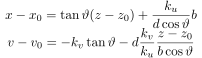$\boldsymbol\Sigma_h$ of the resulting parameters is (HZ04)

$$\boldsymbol\Sigma_h = \left( \sum \mathbf{J}_i^{\top} \boldsymbol\Sigma^{-1}_i \mathbf{J}_i \right)^{+}$$ (9.70)

where $\boldsymbol\Sigma_i$ is the covariance matrix of the noise affecting the individual point.