Scale-Space Representation and SIFT

Harris is a keypoint detector that is not invariant to scale changes. To overcome these limitations, Lindeberg (Lin14,Lin94) introduced the concept of automatic scale selection, which makes it possible to detect keypoints at a given resolution. The image pyramid, a computationally efficient scene representation widely used previously, is in fact a special case of this scale-space representation.

Let $G(x,y;t)$ be the two-dimensional Gaussian with variance $t > 0$, given by

$$G(x,y;t) = \frac{1}{2\pi t} e^{-\frac{x^{2}+y^{2}}{2t} }$$ (6.7)

(see Section 2.2).

The convolution $L(x,y;t)$ of the image 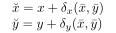$I(x,y)$ with the Gaussian $G(x,y;t)$

$$L(x,y;t) = G(x,y;t) \ast I(x,y)$$ (6.8)

produces the scale-space representation of the image. The variance $t=\sigma^2$ of the Gaussian kernel is called the scale parameter. The image at the degenerate scale $t=0$ is the original image itself.

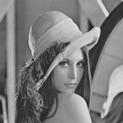
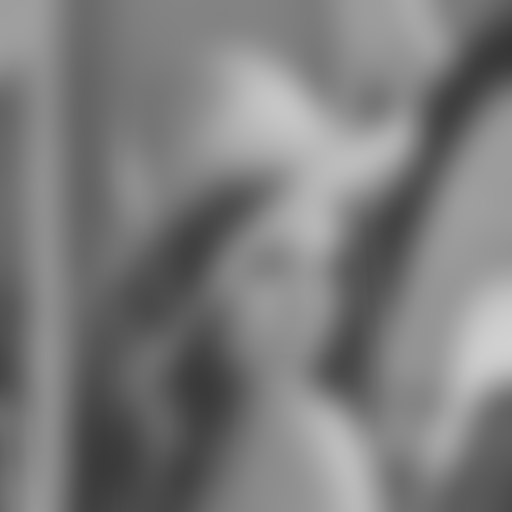
Note that applying a Gaussian filter to an image does not create new structures: all information produced by the filter was already present in the original image.

Figure 6.2: Scale-space representation of an image $512 \times 512$: from the original image $t=0$ to scales 1, 4, 16, 64, and 256.

The scale factor $t$ is a continuous value, but discrete steps are used for computational reasons, usually in exponential sequences such as $t=2^i$ or $t=\frac{1}{2} e^{i}$.

Applying a derivative operator to a scale-space image is, by the commutative property of convolution and differentiation, equivalent to convolving the original image with the derivative of the Gaussian:

$$L_{x^{\alpha}}(\cdot ; t) = \partial_{x^{\alpha}}L(\cdot; t) = (\partial_{x^{\alpha}} g(\cdot; t) ) \ast f(\cdot)$$ (6.9)

where $\alpha$ is multi-index notation for the derivative. Similarly, the definition of any edge or keypoint detector can be extended to any scale factor. Lindeberg's work made it possible to extend Harris corners to scale-invariant cases (the Harris-Laplace and Hessian-Laplace methods (MS02)).

Some useful operators for detecting keypoints include the gradient magnitude $\vert\nabla L\vert$, the Laplacian $\nabla^{2} L$, and the Hessian determinant $\det \mathcal{H}(L)$. All these operators are rotation invariant: the minimum or maximum point exists independently of the image's rotation.

Among these operators, a widely used one for detecting keypoints is the scale-normalized Laplacian of Gaussian (LoG):

$$\nabla_{n}^{2} L(x,y,t) = t(\frac{\partial^2}{\partial x^{2... ...( 1 - \frac{x^2 + y^2}{2t} \right) e^{-\dfrac{x^2 + y^2}{2t} }$$ (6.10)

The LoG operator makes it possible to detect keypoints as local maxima or minima in spatial coordinates and scale.

For example, a circle of radius $r$ has its maximum Laplacian response at scale factor $\sigma = r / \sqrt{2}$.

Figure 6.3: Comparison between the normalized LoG image (a) and the DoG image (b)

(a)	(b)

In the Scale-Invariant Feature Transform (SIFT) algorithm, Lowe (Low04) approximates the Laplacian of Gaussian (LoG) with a Difference of Gaussians (DoG) to improve performance:

$$\begin{array}{rl} D(x,y;\sigma) & = (G(x,y;k\sigma ) - G(x,... ...ma) \\ & \approx (k-1) \sigma^2 LoG(x,y;\sigma) \end{array}$$ (6.11)

This approach is more efficient because the Gaussian image at scale $k\sigma$ can be computed from the Gaussian image at scale $\sigma$ by applying a filter $(k-1)\sigma$, which is smaller and therefore much faster overall than performing the convolution $k\sigma$ with the original image.

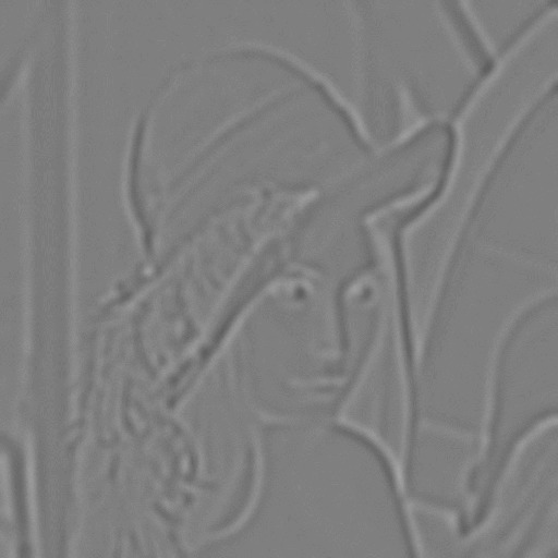
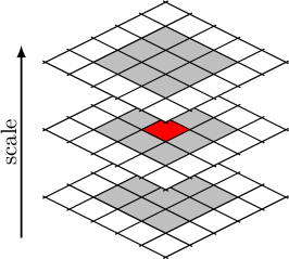
For the LoG, keypoints are local minima or maxima of the Laplacian image in both space and scale. Here, they are the minima and maxima in the difference image between the scale images $\sigma, k\sigma, \ldots, k^n\sigma$ used to process the image (Figure 6.4).

Figure 6.4: Detection of local minima and maxima: for each pixel and each scale, a neighborhood $3\times 3\times 3$ is compared.

With the introduction of the step $k$, the domain of the variable $\sigma$ is effectively divided into discrete logarithmic steps, grouped into octaves, with each octave divided into $S$ sublevels. Thus, $\sigma$ takes the discrete values

$$\sigma(o,s) = \sigma_0 2^{o + \frac{s}{S}} \leftrightarrow k=2^{\frac{1}{S}}$$ (6.12)

where $\sigma_0$ is the base scale factor.

Keypoints found as maxima or minima in scale and space, both of which are discrete, are interpolated using a three-dimensional quadratic fit to locate the keypoint with subpixel and subscale precision.

Between one octave and the next, the image is downsampled by a factor of 2: in addition to the analysis at multiple scales within each octave, the image is processed again in the next octave with its horizontal and vertical dimensions halved. This process is repeated several times.

The second stage of a keypoint detection and matching algorithm is to extract a descriptor for matching, centered on the detected keypoint. To be scale invariant, the descriptor must be extracted at the same scale factor as the keypoint.

To be rotation invariant, the descriptor must be extracted from an image normalized with respect to the dominant orientation estimated in the neighborhood of the point being evaluated.

A descriptor that emphasizes edges in the neighborhood can then be extracted from this image, rotated to the keypoint's scale, and made invariant to illumination.

Among the many variants, PCA-SIFT is worth noting: it uses PCA to reduce the problem to a descriptor with only 36 elements. PCA is used in a prior training stage.