Hough Transform

Figure: Example of the Hough Transform for detecting lines in polar coordinates: accumulator map (top right) of a single point (top left), and accumulator map (bottom right) of a set of collinear points together with outliers (bottom left).

Let $g(\mathbf{x}, \boldsymbol\beta)=0$ be a continuous manifold in $\mathbf {x}$ whose parameters $\boldsymbol\beta \in \mathbb{R}^m$ are to be estimated. To obtain these parameters and completely define the function, a set of coordinates $S = \left\{ \mathbf{x}_1, \ldots, \mathbf{x}_n \right\}$ belonging to the function's locus is available; these coordinates may be noisy and, above all, may potentially be outliers.

The Hough Transform (Hough Transform) is a technique that makes it possible to group a “highly probable” set of points satisfying certain parametric constraints (PIK92).

For every possible point $\boldsymbol\beta^{*}$ in parameter space, it is possible to associate a vote $H(\boldsymbol\beta)$ of the form

$$H(\boldsymbol\beta^{*}) = \left\{ \mathbf{x} : g(\mathbf{x}, \boldsymbol\beta^{*}) = 0, \mathbf{x} \in S \right\}$$ (4.129)

that is, the number of elements of $S$ satisfying the constraint expressed by $g$. The parameter $\boldsymbol\beta^{*}$ that maximizes this vote is the statistically most probable solution to the problem.

Now let the function $p(\mathbf{x}, \boldsymbol\beta)$ be a likelihood index between the pair $(\mathbf{x}, \boldsymbol\beta)$ and the constraint expressed by $g(\mathbf{x}, \boldsymbol\beta)=0$. The function $p$ is normally binary, but, more generally, it can represent a probability. Using the function $p$, the Hough transform $H(\boldsymbol\beta)$ can be constructed incrementally through

$$H(\boldsymbol\beta) = \sum_{i=1}^{n} p(\mathbf{x}_i, \boldsymbol\beta)$$ (4.130)

The Hough transform is the sum of all these functions.

For particular constraints, this approach can be simplified further to reduce computational cost and memory usage.

Let $\beta_1 \ldots \beta_m$ be quantized and bounded parameters to be estimated, and let $f$ and $\beta_1$ be a function and a parameter such that the function $g(\mathbf{x}, \boldsymbol\beta)=0$ can be written as

$$\beta_1 = f(\mathbf{x}, \beta_2 \ldots \beta_m)$$ (4.131)

If the function $g$ can be expressed as in equation (4.131), the discrete Hough transform method can be used to estimate the parameters $\boldsymbol\beta$ representing the “most probable” model among all the points $\mathbf {x}$ provided. For each element $\mathbf {x}$, the parameters $\beta_2 \ldots \beta_m$ can be varied over their range, and the values of $\beta_1$ returned by function (4.131) can be entered into the accumulator image $H(\boldsymbol\beta)$.

In this way, an n-dimensional probability map can be generated using noisy observations $\mathbf {x}$ that may potentially be outliers. Similarly, the Hough method makes it possible to estimate a model in the presence of a mixture of models with different parameters.

The performance of the Hough method improves as the number of constraints increases, dynamically limiting, for example, the range of parameters associated with sample $\mathbf {x}$. The Hough algorithm can be viewed as a degenerate form of template matching.

It is generally useful to use Hough when the model has only two parameters, since it can easily be plotted on a two-dimensional map.

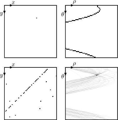
A very common example of the Hough transform is one in which $g$ (the model) is a line, expressed in polar form as in equation (1.82), where the parameters to be determined are $\theta$ and $\rho$: it is clear that, for every pair of points $(x,y)$ and every possible quantized and bounded angle $\theta$ (since the angle is a bounded parameter), there is exactly one $\rho$ satisfying equation (1.82).

It is therefore possible to create a map $H(\theta,\rho)$ in which, for every point $(x,y) \in S$ and every $\theta \in [\theta_{min}, \theta_{max}]$, the element associated with $(\theta, \cos \theta x + \sin \theta y )$ is incremented in the accumulator map, according to the relation satisfying equation (1.82) for the line expressed in polar coordinates.