


Next: Gradient Descent Up: Optimization Methods Previous: Optimization Methods
The problem of finding the minima of a function can be reduced to the problem of finding the zeros of a function, specifically the first derivative of the cost function  .
.
Let
 be a differentiable multivariate function whose
 in a Taylor series locally around a suitable point
  gives
gives
 is the
  matrix, the Jacobian of function evaluated at .
The objective is to modify the value of by an amount
 such that the cost function evaluated at
 is exactly zero.
Ignoring terms of order higher than
is exactly zero.
Ignoring terms of order higher than
 , the estimate of
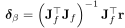
that, to first order, brings the function closer to zero is the solution of the linear system (4.30) subject to the condition (4.29), namely
, the estimate of
that, to first order, brings the function closer to zero is the solution of the linear system (4.30) subject to the condition (4.29), namely
has full rank, is a simple, possibly overdetermined linear system that can be solved using one of the techniques presented in Section 1.1.
The idea behind iterative methods is to modify the point  by the quantity

 |
(4.32) |
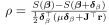 , computed so as to progressively approach the zero of the function.
In the single-variable case  , Newton's method reduces to
 |
(4.33) |
In numerical analysis, this is the so-called Newton method (or Newton-Raphson method) for finding the zeros of a function.
The maxima and minima of a function are points at which the gradient can be set to zero.
This technique can therefore be applied to find the maxima and minima of a function
 by defining
 |
(4.34) |
 is the gradient function
 , while
 is the Hessian matrix
  ; these are the gradient and Hessian functions of
  evaluated at .
Newton's update of the point therefore becomes
evaluated at .
Newton's update of the point therefore becomes
 in the neighborhood of with a quadratic function.
If is a quadratic function, convergence is guaranteed in a single iteration.
in the neighborhood of with a quadratic function.
If is a quadratic function, convergence is guaranteed in a single iteration.
Now, in the specific case of optimization methods, the function is the cost function
 .
Therefore, when the Hessian matrix of
is nonsingular, the parameter update equation
.
Therefore, when the Hessian matrix of
is nonsingular, the parameter update equation
Paolo medici



